Bernoulli sampling

The most basic Bernoulli method generates n random variates to extract a sample from a population of n items. Suppose you want to extract a given percentage pct of the population. The algorithm can be described as follows:[2]

for each item in the set
    generate a random non-negative integer R
    if (R mod 100) < pct then
        select item

Scaled f(k, n, 0.2) for four values of n.

A percentage of 20%, say, is usually expressed as a probability p=0.2. In that case, random variates are generated in the unit interval. After running the algorithm, a sample of size k will have been selected. One would expect to have ${\displaystyle k\approx n\cdot p}$, which is more and more likely as n grows. In fact, It is possible to calculate the probability of obtaining a sample size of k by the Binomial distribution:

$${\displaystyle f(k,n,p)={\binom {n}{k}}p^{k}(1-p)^{n-k}}$$

On the left this function is shown for four values of ${\displaystyle n}$ and ${\displaystyle p=0.2}$. In order to compare the values for different values of ${\displaystyle n}$, the ${\displaystyle k}$'s in abscissa are scaled from ${\displaystyle \left[0,n\right]}$ to the unit interval, while the value of the function, in ordinate, is multiplied by the inverse, so that the area under the graph maintains the same value —that area is related to the corresponding cumulative distribution function. The values are shown in logarithmic scale.

Values of n such that a Bernoulli sample size is within error in 95% of cases.

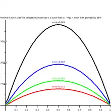
On the right the minimum values of ${\displaystyle n}$ that satisfy given error bounds with 95% probability. Given an error, the set of ${\displaystyle k}$'s within bounds can be described as follows:

$${\displaystyle K_{n,p}=\left\{k\in \mathbb {N}$$ :\left\vert {\frac {k}{n}}-p\right\vert <\mathrm {error} \right\}}

The probability to end up within ${\displaystyle K}$ is given again by the binomial distribution as:

$${\displaystyle \sum _{k\in K}f(k,n,p).}$$

The picture shows the lowest values of ${\displaystyle n}$ such that the sum is at least 0.95. For ${\displaystyle p=0.0}$ and ${\displaystyle p=1.00}$ the algorithm delivers exact results for all ${\displaystyle n}$'s. The ${\displaystyle p}$'s in between are obtained by bisection. Note that, if ${\displaystyle 100\cdot p}$ is an integer percentage, ${\displaystyle \mathrm {error} =0.005}$, guarantees that ${\displaystyle 100\cdot k/n=100\cdot p}$. Values as high as ${\displaystyle n=38400}$ can be required for such an exact match.

• Poisson sampling
• Bernoulli trial
• Bernoulli process
• Sampling design

• Faster Random Samples With Gap Sampling

References

- Carl-Erik Sarndal; Bengt Swensson; Jan Wretman (1992). Model Assisted Survey Sampling. ISBN 978-0-387-97528-3.
- Voratas Kachitvichyanukul; Bruce W. Schmeise (1 February 1988). "Binomial Random Variate Generation". Communications of the ACM. 31 (2): 216–222. doi:10.1145/42372.42381. S2CID 18698828.