Catastrophe theory
In mathematics, catastrophe theory is a branch of bifurcation theory in the study of dynamical systems; it is also a particular special case of more general singularity theory in geometry.
Bifurcation theory studies and classifies phenomena characterized by sudden shifts in behavior arising from small changes in circumstances, analysing how the qualitative nature of equation solutions depends on the parameters that appear in the equation. This may lead to sudden and dramatic changes, for example the unpredictable timing and magnitude of a landslide.
Catastrophe theory originated with the work of the French mathematician René Thom in the 1960s, and became very popular due to the efforts of Christopher Zeeman in the 1970s. It considers the special case where the long-run stable equilibrium can be identified as the minimum of a smooth, well-defined potential function (Lyapunov function). Small changes in certain parameters of a nonlinear system can cause equilibria to appear or disappear, or to change from attracting to repelling and vice versa, leading to large and sudden changes of the behaviour of the system. However, examined in a larger parameter space, catastrophe theory reveals that such bifurcation points tend to occur as part of well-defined qualitative geometrical structures.
In the late 1970s, applications of catastrophe theory to areas outside its scope began to be criticized, especially in biology and social sciences.[1][2] Zahler and Sussmann, in a 1977 article in Nature, referred to such applications as being "characterised by incorrect reasoning, far-fetched assumptions, erroneous consequences, and exaggerated claims".[3] As a result, catastrophe theory has become less popular in applications.[4]
Elementary catastrophes
Catastrophe theory analyzes degenerate critical points of the potential function — points where not just the first derivative, but one or more higher derivatives of the potential function are also zero. These are called the germs of the catastrophe geometries. The degeneracy of these critical points can be unfolded by expanding the potential function as a Taylor series in small perturbations of the parameters.
When the degenerate points are not merely accidental, but are structurally stable, the degenerate points exist as organising centres for particular geometric structures of lower degeneracy, with critical features in the parameter space around them. If the potential function depends on two or fewer active variables, and four or fewer active parameters, then there are only seven generic structures for these bifurcation geometries, with corresponding standard forms into which the Taylor series around the catastrophe germs can be transformed by diffeomorphism (a smooth transformation whose inverse is also smooth). These seven fundamental types are now presented, with the names that Thom gave them.
Potential functions of one active variable
Catastrophe theory studies dynamical systems that describe the evolution[5] of a state variable over time :
In the above equation, is referred to as the potential function, and is often a vector or a scalar which parameterise the potential function. The value of may change over time, and it can also be referred to as the control variable. In the following examples, parameters like are such controls.
Fold catastrophe
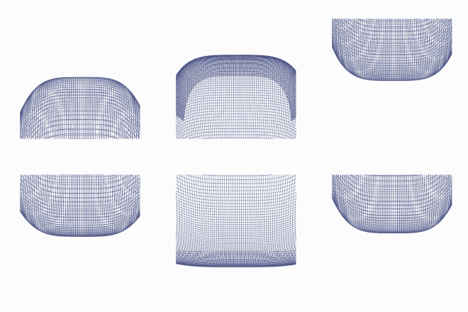
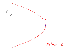
When a < 0, the potential V has two extrema - one stable, and one unstable. If the parameter a is slowly increased, the system can follow the stable minimum point. But at a = 0 the stable and unstable extrema meet, and annihilate. This is the bifurcation point. At a > 0 there is no longer a stable solution. If a physical system is followed through a fold bifurcation, one therefore finds that as a reaches 0, the stability of the a < 0 solution is suddenly lost, and the system will make a sudden transition to a new, very different behaviour. This bifurcation value of the parameter a is sometimes called the "tipping point".
Cusp catastrophe
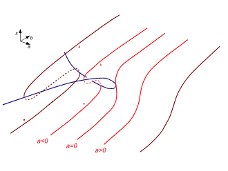 Diagram of cusp catastrophe, showing curves (brown, red) of x satisfying dV/dx = 0 for parameters (a,b), drawn for parameter b continuously varied, for several values of parameter a. Outside the cusp locus of bifurcations (blue), for each point (a,b) in parameter space there is only one extremising value of x. Inside the cusp, there are two different values of x giving local minima of V(x) for each (a,b), separated by a value of x giving a local maximum. | |
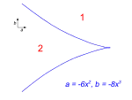 Cusp shape in parameter space (a,b) near the catastrophe point, showing the locus of fold bifurcations separating the region with two stable solutions from the region with one. |
 Pitchfork bifurcation at a = 0 on the surface b = 0 |
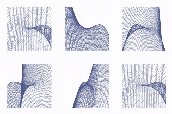 Cusp catastrophe, with surface .
The cusp geometry is very common when one explores what happens to a fold bifurcation if a second parameter, b, is added to the control space. Varying the parameters, one finds that there is now a curve (blue) of points in (a,b) space where stability is lost, where the stable solution will suddenly jump to an alternate outcome.
But in a cusp geometry the bifurcation curve loops back on itself, giving a second branch where this alternate solution itself loses stability, and will make a jump back to the original solution set. By repeatedly increasing b and then decreasing it, one can therefore observe hysteresis loops, as the system alternately follows one solution, jumps to the other, follows the other back, and then jumps back to the first.
However, this is only possible in the region of parameter space a < 0. As a is increased, the hysteresis loops become smaller and smaller, until above a = 0 they disappear altogether (the cusp catastrophe), and there is only one stable solution.
One can also consider what happens if one holds b constant and varies a. In the symmetrical case b = 0, one observes a pitchfork bifurcation as a is reduced, with one stable solution suddenly splitting into two stable solutions and one unstable solution as the physical system passes to a < 0 through the cusp point (0,0) (an example of spontaneous symmetry breaking). Away from the cusp point, there is no sudden change in a physical solution being followed: when passing through the curve of fold bifurcations, all that happens is an alternate second solution becomes available.
A famous suggestion is that the cusp catastrophe can be used to model the behaviour of a stressed dog, which may respond by becoming cowed or becoming angry.[6] The suggestion is that at moderate stress (a > 0), the dog will exhibit a smooth transition of response from cowed to angry, depending on how it is provoked. But higher stress levels correspond to moving to the region (a < 0). Then, if the dog starts cowed, it will remain cowed as it is irritated more and more, until it reaches the 'fold' point, when it will suddenly, discontinuously snap through to angry mode. Once in 'angry' mode, it will remain angry, even if the direct irritation parameter is considerably reduced.
A simple mechanical system, the "Zeeman Catastrophe Machine", nicely illustrates a cusp catastrophe. In this device, smooth variations in the position of the end of a spring can cause sudden changes in the rotational position of an attached wheel.[7]
Catastrophic failure of a complex system with parallel redundancy can be evaluated based on the relationship between local and external stresses. The model of the structural fracture mechanics is similar to the cusp catastrophe behavior. The model predicts reserve ability of a complex system.
Other applications include the outer sphere electron transfer frequently encountered in chemical and biological systems,[8] modelling the dynamics of cloud condensation nuclei in the atmosphere,[9] and modelling real estate prices.[10]
Fold bifurcations and the cusp geometry are by far the most important practical consequences of catastrophe theory. They are patterns which reoccur again and again in physics, engineering and mathematical modelling. They produce the strong gravitational lensing events and provide astronomers with one of the methods used for detecting black holes and the dark matter of the universe, via the phenomenon of gravitational lensing producing multiple images of distant quasars.[11]
The remaining simple catastrophe geometries are very specialised in comparison, and presented here only for curiosity value.
Swallowtail catastrophe
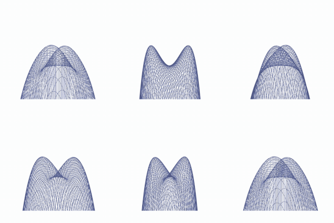
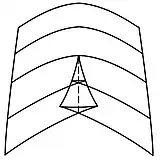
The control parameter space is three-dimensional. The bifurcation set in parameter space is made up of three surfaces of fold bifurcations, which meet in two lines of cusp bifurcations, which in turn meet at a single swallowtail bifurcation point.
As the parameters go through the surface of fold bifurcations, one minimum and one maximum of the potential function disappear. At the cusp bifurcations, two minima and one maximum are replaced by one minimum; beyond them the fold bifurcations disappear. At the swallowtail point, two minima and two maxima all meet at a single value of x. For values of a > 0, beyond the swallowtail, there is either one maximum-minimum pair, or none at all, depending on the values of b and c. Two of the surfaces of fold bifurcations, and the two lines of cusp bifurcations where they meet for a < 0, therefore disappear at the swallowtail point, to be replaced with only a single surface of fold bifurcations remaining. Salvador Dalí's last painting, The Swallow's Tail, was based on this catastrophe.
Butterfly catastrophe
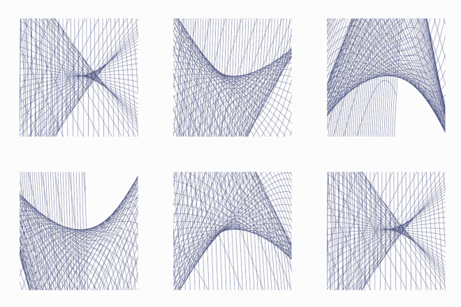
Depending on the parameter values, the potential function may have three, two, or one different local minima, separated by the loci of fold bifurcations. At the butterfly point, the different 3-surfaces of fold bifurcations, the 2-surfaces of cusp bifurcations, and the lines of swallowtail bifurcations all meet up and disappear, leaving a single cusp structure remaining when a > 0.
Potential functions of two active variables

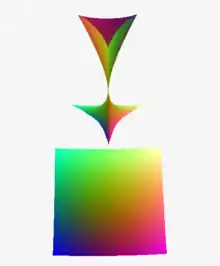
Umbilic catastrophes are examples of corank 2 catastrophes. They can be observed in optics in the focal surfaces created by light reflecting off a surface in three dimensions and are intimately connected with the geometry of nearly spherical surfaces: umbilical point. Thom proposed that the hyperbolic umbilic catastrophe modeled the breaking of a wave and the elliptical umbilic modeled the creation of hair-like structures.
Hyperbolic umbilic catastrophe
Elliptic umbilic catastrophe
Parabolic umbilic catastrophe
Arnold's notation
Vladimir Arnold gave the catastrophes the ADE classification, due to a deep connection with simple Lie groups.
- A0 - a non-singular point: .
- A1 - a local extremum, either a stable minimum or unstable maximum .
- A2 - the fold
- A3 - the cusp
- A4 - the swallowtail
- A5 - the butterfly
- Ak - a representative of an infinite sequence of one variable forms
- D4− - the elliptical umbilic
- D4+ - the hyperbolic umbilic
- D5 - the parabolic umbilic
- Dk - a representative of an infinite sequence of further umbilic forms
- E6 - the symbolic umbilic
- E7
- E8
There are objects in singularity theory which correspond to most of the other simple Lie groups.
See also
References
- Murray, Stacey R. "The Rise and Fall of Catastrophe Theory". Encyclopedia.com. Retrieved 2 November 2021.
- Horgan, John (2015). The End of Science: Facing the Limits of Knowledge in the Twilight of the Scientific Age. New York: Basic Books. p. 213. ISBN 978-0-465-05085-7.
- Zahler, Raphael S.; Sussmann, Hector J. (1977). "Claims and accomplishments of applied catastrophe theory". Nature. 269 (5631): 759–763. Bibcode:1977Natur.269..759Z. doi:10.1038/269759a0. ISSN 1476-4687. S2CID 4205198. Retrieved 2021-11-02.
- Rosser, J. Barkley (October 2007). "The rise and fall of catastrophe theory applications in economics: Was the baby thrown out with the bathwater?". Journal of Economic Dynamics and Control. 31 (10): 3255–3280. doi:10.1016/j.jedc.2006.09.013.
- Wagenmakers, E. J.; van der Maas, H. L. J.; Molenaar, P. C. M. (2005). "Fitting the cusp catastrophe model". Encyclopedia of Statistics in Behavioral Science.
- E.C. Zeeman, Catastrophe Theory, Scientific American, April 1976; pp. 65–70, 75–83
- Cross, Daniel J., Interactive rendering of Zeeman's Catastrophe Machine
- Xu, F (1990). "Application of catastrophe theory to the ∆G≠ to -∆G relationship in electron transfer reactions". Zeitschrift für Physikalische Chemie. Neue Folge. 166: 79–91. doi:10.1524/zpch.1990.166.Part_1.079. S2CID 101078817.
- Arabas, S; Shima, S. (2017). "On the CCN (de)activation nonlinearities". Nonlinear Processes in Geophysics. 24 (3): 535–542. arXiv:1608.08187. Bibcode:2017NPGeo..24..535A. doi:10.5194/npg-24-535-2017. S2CID 24669360.
- Bełej, Mirosław; Kulesza, Sławomir (2012). "Modeling the Real Estate Prices in Olsztyn under Instability Conditions". Folia Oeconomica Stetinensia. 11 (1): 61–72. doi:10.2478/v10031-012-0008-7.
- A.O. Petters, H. Levine and J. Wambsganss, Singularity Theory and Gravitational Lensing", Birkhäuser Boston (2001)
Bibliography
- Arnold, Vladimir Igorevich (1992) Catastrophe Theory, 3rd ed. Berlin: Springer-Verlag
- V. S. Afrajmovich, V. I. Arnold, et al., Bifurcation Theory And Catastrophe Theory, ISBN 3-540-65379-1
- Bełej,M. Kulesza, S. (2013) M"odeling the Real Estate Prices in Olsztyn under Instability Conditions", Folia Oeconomica Stetinensia 11(1): 61–72, ISSN (Online) 1898–0198, ISSN (Print) 1730–4237, doi:10.2478/v10031-012-0008-7
- Castrigiano, Domenico P. L. and Hayes, Sandra A. (2004) Catastrophe Theory, second edition, Boulder: Westview ISBN 0-8133-4126-4
- Gilmore, Robert (1993) Catastrophe Theory for Scientists and Engineers, New York: Dover
- Petters, Arlie O., Levine, Harold and Wambsganss, Joachim (2001) Singularity Theory and Gravitational Lensing, Boston: Birkhäuser ISBN 0-8176-3668-4
- Postle, Denis (1980) Catastrophe Theory – Predict and avoid personal disasters, Fontana Paperbacks ISBN 0-00-635559-5
- Poston, Tim and Stewart, Ian (1998) Catastrophe: Theory and Its Applications, New York: Dover ISBN 0-486-69271-X
- Sanns, Werner (2000) Catastrophe Theory with Mathematica: A Geometric Approach, Germany: DAV
- Saunders, Peter Timothy (1980) An Introduction to Catastrophe Theory, Cambridge, England: Cambridge University Press
- Thom, René (1989) Structural Stability and Morphogenesis: An Outline of a General Theory of Models, Reading, MA: Addison-Wesley ISBN 0-201-09419-3
- Woodcock, Alexander Edward Richard and Davis, Monte. (1978) Catastrophe Theory, New York: E. P. Dutton ISBN 0-525-07812-6
- Zeeman, E.C. (1977) Catastrophe Theory-Selected Papers 1972–1977, Reading, MA: Addison-Wesley