Chebyshev filter

The frequency response of a fourth-order type I Chebyshev low-pass filter with ${\displaystyle \varepsilon =1}$

Type I Chebyshev filters are the most common types of Chebyshev filters. The gain (or amplitude) response, ${\displaystyle G_{n}(\omega )}$, as a function of angular frequency ${\displaystyle \omega }$ of the ${\displaystyle n}$th-order low-pass filter is equal to the absolute value of the transfer function ${\displaystyle H_{n}(s)}$ evaluated at ${\displaystyle s=j\omega }$:

${\displaystyle G_{n}(\omega )=\left|H_{n}(j\omega )\right|={\frac {1}{\sqrt {1+\varepsilon ^{2}T_{n}^{2}(\omega /\omega _{0})}}}}$

where ${\displaystyle \varepsilon }$ is the ripple factor, ${\displaystyle \omega _{0}}$ is the cutoff frequency and ${\displaystyle T_{n}}$ is a Chebyshev polynomial of the ${\displaystyle n}$th order.

The passband exhibits equiripple behavior, with the ripple determined by the ripple factor ${\displaystyle \varepsilon }$. In the passband, the Chebyshev polynomial alternates between -1 and 1 so the filter gain alternate between maxima at ${\displaystyle G=1}$ and minima at ${\displaystyle G=1/{\sqrt {1+\varepsilon ^{2}}}}$.

The ripple factor ε is thus related to the passband ripple δ in decibels by:

${\displaystyle \varepsilon ={\sqrt {10^{\delta /10}-1}}.}$

At the cutoff frequency ${\displaystyle \omega _{0}}$ the gain again has the value ${\displaystyle 1/{\sqrt {1+\varepsilon ^{2}}}}$ but continues to drop into the stopband as the frequency increases. This behavior is shown in the diagram on the right. The common practice of defining the cutoff frequency at −3 dB is usually not applied to Chebyshev filters; instead the cutoff is taken as the point at which the gain falls to the value of the ripple for the final time.

The 3 dB frequency ${\displaystyle \omega _{H}}$ is related to ${\displaystyle \omega _{0}}$ by:

${\displaystyle \omega _{H}=\omega _{0}\cosh \left({\frac {1}{n}}\cosh ^{-1}{\frac {1}{\varepsilon }}\right).}$

The order of a Chebyshev filter is equal to the number of reactive components (for example, inductors) needed to realize the filter using analog electronics.

An even steeper roll-off can be obtained if ripple is allowed in the stopband, by allowing zeros on the ${\displaystyle \omega }$-axis in the complex plane. While this produces near-infinite suppression at and near these zeros (limited by the quality factor of the components, parasitics, and related factors), overall suppression in the stopband is reduced. The result is called an elliptic filter, also known as a Cauer filter.

Poles and zeroes

Log of the absolute value of the gain of an 8th-order Chebyshev type I filter in complex frequency space (s = σ + jω) with ε = 0.1 and ${\displaystyle \omega _{0}=1}$. The white spots are poles and are arranged on an ellipse with a semi-axis of 0.3836... in σ and 1.071... in ω. The transfer function poles are those poles in the left half plane. Black corresponds to a gain of 0.05 or less, white corresponds to a gain of 20 or more.

For simplicity, it is assumed that the cutoff frequency is equal to unity. The poles ${\displaystyle (\omega _{pm})}$ of the gain function of the Chebyshev filter are the zeroes of the denominator of the gain function. Using the complex frequency ${\displaystyle s}$, these occur when:

${\displaystyle 1+\varepsilon ^{2}T_{n}^{2}(-js)=0.\,}$

Defining ${\displaystyle -js=\cos(\theta )}$ and using the trigonometric definition of the Chebyshev polynomials yields:

${\displaystyle 1+\varepsilon ^{2}T_{n}^{2}(\cos(\theta ))=1+\varepsilon ^{2}\cos ^{2}(n\theta )=0.\,}$

Solving for ${\displaystyle \theta }$

${\displaystyle \theta ={\frac {1}{n}}\arccos \left({\frac {\pm j}{\varepsilon }}\right)+{\frac {m\pi }{n}}}$

where the multiple values of the arc cosine function are made explicit using the integer index ${\displaystyle m}$. The poles of the Chebyshev gain function are then:

${\displaystyle s_{pm}=j\cos(\theta )\,}$

${\displaystyle =j\cos \left({\frac {1}{n}}\arccos \left({\frac {\pm j}{\varepsilon }}\right)+{\frac {m\pi }{n}}\right).}$

Using the properties of the trigonometric and hyperbolic functions, this may be written in explicitly complex form:

${\displaystyle s_{pm}^{\pm }=\pm \sinh \left({\frac {1}{n}}\mathrm {arsinh} \left({\frac {1}{\varepsilon }}\right)\right)\sin(\theta _{m})}$

${\displaystyle +j\cosh \left({\frac {1}{n}}\mathrm {arsinh} \left({\frac {1}{\varepsilon }}\right)\right)\cos(\theta _{m})}$

where ${\displaystyle m=1,2,...,n}$ and

${\displaystyle \theta _{m}={\frac {\pi }{2}}\,{\frac {2m-1}{n}}.}$

This may be viewed as an equation parametric in ${\displaystyle \theta _{n}}$ and it demonstrates that the poles lie on an ellipse in ${\displaystyle s}$-space centered at ${\displaystyle s=0}$ with a real semi-axis of length ${\displaystyle \sinh(\mathrm {arsinh} (1/\varepsilon )/n)}$ and an imaginary semi-axis of length of ${\displaystyle \cosh(\mathrm {arsinh} (1/\varepsilon )/n).}$

The group delay

Gain and group delay of a 5th-order type I Chebyshev filter with ε = 0.5.

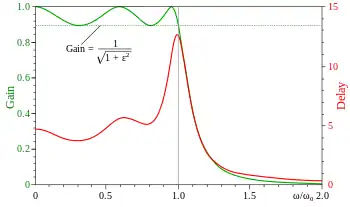
The group delay is defined as the derivative of the phase with respect to angular frequency and is a measure of the distortion in the signal introduced by phase differences for different frequencies.

${\displaystyle \tau _{g}=-{\frac {d}{d\omega }}\arg(H(j\omega ))}$

The gain and the group delay for a 5th-order type I Chebyshev filter with ε=0.5 are plotted in the graph on the left. It can be seen that there are ripples in the gain and the group delay in the passband but not in the stopband.

Pass band cutoff attenuation for Chebyshev filters is usually the same as the pass band ripple attenuation, set by the ${\displaystyle \varepsilon }$ computation above. However, many applications such as diplexers and triplexers, require a cutoff attenuation of -3.0103 dB in order to obtain the needed reflections. Other specialized applications may require other specific values for cutoff attenuation for various reasons. It is therefore useful to have a means available of setting the Chebyshev pass band cutoff attenuation independently of the pass band ripple attenuation, such as -1 dB, -10 dB, etc. The cutoff attenuation is set by frequency scaling the denominator of the transfer function. This can be approximated by interpolating Chebyshev filter cutoff attenuation tables, or calculated precisely with Newton's method.

The denominator may be frequency scaled by using a scaling factor that we will refer to as ${\displaystyle \omega _{c}}$. The frequency scaled denominator of the Chebyshev transfer function may be rewritten for the ${\displaystyle n=3}$ case in terms of frequency scaling variable ${\displaystyle \omega _{c}}$ as follows:

${\displaystyle H(s)={\frac {C}{(s/\omega _{c})^{3}+A(s/\omega _{c})^{2}+Bs/\omega _{c}+C}}}$

The task for modifying ${\displaystyle H(s)}$ to is to find an ${\displaystyle \omega _{c}}$ that results in the desired attenuation at 1 radian/s for the normalized transfer function. Newton's method can be easily summarized to do this by its basic definition:

${\displaystyle \omega _{a}=\omega _{a}+(|H(j\omega _{a})|-{\text{DesiredAttenuation}})/(d|H(j\omega _{a})|/dj\omega _{a})}$

through successive iterations of ${\displaystyle \omega _{a}}$ until ${\displaystyle \omega _{a}}$is the frequency that attenuates ${\displaystyle |H(j\omega _{a})|}$to the desired attenuation at 1 radian/s.

While the above summary may be concise and easily understood, the mechanics of obtaining an accurate derivative of the magnitude function along the ${\displaystyle j\omega }$ axis may be problematic. Digital techniques may be used, but it is generally better to apply Newton's method with continuous functions, if possible, so as to maximize accuracy. Therefore, it is useful to modify the expression to eliminate excess mathematical functions by making the following alterations:

1) Multiply ${\displaystyle H(s)}$ by ${\displaystyle H(-s)}$ to obtain ${\displaystyle H(s)H(-s)}$. This will eliminate complex numerical results when evaluating ${\displaystyle |H(s)H(-s)|}$ by removing the odd order terms in the polynomial.

2) In ${\displaystyle H(s)H(-s)}$, negate all terms of ${\displaystyle s^{n}}$ when ${\displaystyle n+2}$ is divisible by 4. That would be ${\displaystyle s^{2}}$, ${\displaystyle s^{6}}$, ${\displaystyle s^{10}}$, and so on. We will call the modified function ${\displaystyle H_{2}(s)H_{2}(-s)}$, and this modification will allow the use of real numbers instead of complex numbers when evaluating the polynomial and its derivative. That is, we can now use the real ${\displaystyle \omega _{a}}$in place of the complex ${\displaystyle j\omega _{a}}$

3) Convert the desired attenuation in dB to an arithmetic value using ${\displaystyle atten_{arith}=10^{atten_{dB}/20}}$. For example, -3.0103 dB is .7071, -1 dB is .8913 ans so on. This simplifies the derivative evaluation.

4) Square the resulting arithmetic attenuation to correlate with the squaring of the ${\displaystyle H(s)}$ function.

5) Calculate the modified ${\displaystyle H_{2}(\omega _{a})H_{2}(-\omega _{a})}$ in Newton's method using the real value, ${\displaystyle \omega _{a}}$. Always take the absolute value.

6) Calculate the derivative the modified ${\displaystyle H_{2}(\omega _{a})H_{2}(-\omega _{a})}$ with respect to the real value, ${\displaystyle \omega _{a}}$. Negate the derivative computation to account for the effects due to the modifications made to create ${\displaystyle H_{2}(\omega _{a})H_{2}(-\omega _{a})}$. DO NOT take the absolute value of the derivative.

When steps 1) through 4) are compete, Newton's method expression my be written:

${\displaystyle \omega _{a}=\omega _{a}+([H_{2}(\omega _{a})H_{2}(-\omega _{a})]-{\text{DesiredAttenuation}})/(d[H_{2}(\omega _{a})H_{2}(-\omega _{a})]/d\omega _{a})}$

using a real value for ${\displaystyle \omega _{a}}$with no complex arithmetic needed. The movement of ${\displaystyle \omega _{a}}$ should be limited to prevent it from going less than 1 radian/s and into the ripple frequencies early in the iterations for increased reliability. When complete, invert ${\displaystyle \omega _{a}}$to obtain an ${\displaystyle \omega _{c}}$that can be used to scale the original ${\displaystyle H(s)}$ transfer function denominator. The attenuation of ${\displaystyle H(s/\omega _{c})}$ will then be virtually the exact desired value at 1 radian/s. If performed properly, only a handful of iterations are needed to set the attenuation through a wide range of desired attenuation values for both small and very large order Chebyshev filters.

The frequency response of a fifth-order type II Chebyshev low-pass filter with ${\displaystyle \varepsilon =0.01}$

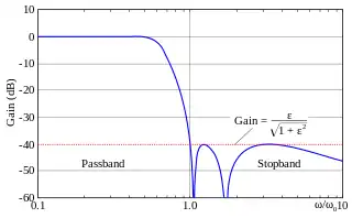
Also known as inverse Chebyshev filters, the Type II Chebyshev filter type is less common because it does not roll off as fast as Type I, and requires more components. It has no ripple in the passband, but does have equiripple in the stopband. The gain is:

${\displaystyle G_{n}(\omega )={\frac {1}{\sqrt {1+{\frac {1}{\varepsilon ^{2}T_{n}^{2}(\omega _{0}/\omega )}}}}}={\sqrt {\frac {\varepsilon ^{2}T_{n}^{2}(\omega _{0}/\omega )}{1+\varepsilon ^{2}T_{n}^{2}(\omega _{0}/\omega )}}}.}$

In the stopband, the Chebyshev polynomial oscillates between -1 and 1 so that the gain will oscillate between zero and

${\displaystyle {\frac {1}{\sqrt {1+{\frac {1}{\varepsilon ^{2}}}}}}}$

and the smallest frequency at which this maximum is attained is the cutoff frequency ${\displaystyle \omega _{o}}$. The parameter ε is thus related to the stopband attenuation γ in decibels by:

${\displaystyle \varepsilon ={\frac {1}{\sqrt {10^{\gamma /10}-1}}}.}$

For a stopband attenuation of 5 dB, ε = 0.6801; for an attenuation of 10 dB, ε = 0.3333. The frequency f₀ = ω₀/2π is the cutoff frequency. The 3 dB frequency f_H is related to f₀ by:

${\displaystyle f_{H}={\frac {f_{0}}{\cosh \left({\frac {1}{n}}\cosh ^{-1}{\frac {1}{\varepsilon }}\right)}}.}$

Poles and zeroes

Log of the absolute value of the gain of an 8th order Chebyshev type II filter in complex frequency space (s=σ+jω) with ε = 0.1 and ${\displaystyle \omega _{0}=1}$. The white spots are poles and the black spots are zeroes. All 16 poles are shown. Each zero has multiplicity of two, and 12 zeroes are shown and four are located outside the picture, two on the positive ω axis, and two on the negative. The poles of the transfer function are poles on the left half plane and the zeroes of the transfer function are the zeroes, but with multiplicity 1. Black corresponds to a gain of 0.05 or less, white corresponds to a gain of 20 or more.

Assuming that the cutoff frequency is equal to unity, the poles ${\displaystyle (\omega _{pm})}$ of the gain of the Chebyshev filter are the zeroes of the denominator of the gain:

${\displaystyle 1+\varepsilon ^{2}T_{n}^{2}(-1/js_{pm})=0.}$

The poles of gain of the type II Chebyshev filter are the inverse of the poles of the type I filter:

${\displaystyle {\frac {1}{s_{pm}^{\pm }}}=\pm \sinh \left({\frac {1}{n}}\mathrm {arsinh} \left({\frac {1}{\varepsilon }}\right)\right)\sin(\theta _{m})}$

${\displaystyle \qquad +j\cosh \left({\frac {1}{n}}\mathrm {arsinh} \left({\frac {1}{\varepsilon }}\right)\right)\cos(\theta _{m})}$

where ${\displaystyle m=1,2,...n}$. The zeroes ${\displaystyle (\omega _{zm})}$ of the type II Chebyshev filter are the zeroes of the numerator of the gain:

${\displaystyle \varepsilon ^{2}T_{n}^{2}(-1/js_{zm})=0.\,}$

The zeroes of the type II Chebyshev filter are therefore the inverse of the zeroes of the Chebyshev polynomial.

${\displaystyle 1/s_{zm}=-j\cos \left({\frac {\pi }{2}}\,{\frac {2m-1}{n}}\right)}$

for ${\displaystyle m=1,2,...n}$.

The group delay

Gain and group delay of a fifth-order type II Chebyshev filter with ε = 0.1.

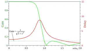
The gain and the group delay for a fifth-order type II Chebyshev filter with ε=0.1 are plotted in the graph on the left. It can be seen that there are ripples in the gain in the stopband but not in the pass band.

The following illustration shows the Chebyshev filters next to other common filter types obtained with the same number of coefficients (fifth order):

Chebyshev filters are sharper than the Butterworth filter; they are not as sharp as the elliptic one, but they show fewer ripples over the bandwidth.

• Bessel filter
• Butterworth filter
• Chebyshev nodes
• Chebyshev polynomial
• Comb filter
• Elliptic filter
• Filter design

• Media related to Chebyshev filters at Wikimedia Commons

References

- Daniels, Richard W. (1974). Approximation Methods for Electronic Filter Design. New York: McGraw-Hill. ISBN 0-07-015308-6.
- Lutovac, Miroslav D.; Lutovac, D.; Tošić, Dejan V.; Evans, Brian Lawrence (2001). Filter Design for Signal Processing Using MATLAB and Mathematica. Prentice Hall. ISBN 9780201361308.
- Weinberg, Louis; Slepian, Paul (June 1960). "Takahasi's Results on Tchebycheff and Butterworth Ladder Networks". IRE Transactions on Circuit Theory. 7 (2): 88–101. doi:10.1109/TCT.1960.1086643.
- Williams, Arthur B.; Taylors, Fred J. (1988). Electronic Filter Design Handbook. New York: McGraw-Hill. ISBN 0-07-070434-1.
- Matthaei, George L.; Young, Leo; Jones, E. M. T. (1980). Microwave Filters, Impedance-Matching Networks, and Coupling Structures. Norwood, MA: Artech House. ISBN 0-89-006099-1.
External links