Decomposition of time series

This is an important technique for all types of time series analysis, especially for seasonal adjustment.[2] It seeks to construct, from an observed time series, a number of component series (that could be used to reconstruct the original by additions or multiplications) where each of these has a certain characteristic or type of behavior. For example, time series are usually decomposed into:

• ${\displaystyle T_{t}}$, the trend component at time t, which reflects the long-term progression of the series (secular variation). A trend exists when there is a persistent increasing or decreasing direction in the data. The trend component does not have to be linear.[1]
• ${\displaystyle C_{t}}$, the cyclical component at time t, which reflects repeated but non-periodic fluctuations. The duration of these fluctuations depend on the nature of the time series.
• ${\displaystyle S_{t}}$, the seasonal component at time t, reflecting seasonality (seasonal variation). A seasonal pattern exists when a time series is influenced by seasonal factors. Seasonality occurs over a fixed and known period (e.g., the quarter of the year, the month, or day of the week).[1]
• ${\displaystyle I_{t}}$, the irregular component (or "noise") at time t, which describes random, irregular influences. It represents the residuals or remainder of the time series after the other components have been removed.

Hence a time series using an additive model can be thought of as

${\displaystyle y_{t}=T_{t}+C_{t}+S_{t}+I_{t},}$

whereas a multiplicative model would be

${\displaystyle y_{t}=T_{t}\times C_{t}\times S_{t}\times I_{t}.\,}$

An additive model would be used when the variations around the trend do not vary with the level of the time series whereas a multiplicative model would be appropriate if the trend is proportional to the level of the time series.[3]

Sometimes the trend and cyclical components are grouped into one, called the trend-cycle component. The trend-cycle component can just be referred to as the "trend" component, even though it may contain cyclical behavior.[3] For example, a seasonal decomposition of time series by Loess (STL)[4] plot decomposes a time series into seasonal, trend and irregular components using loess and plots the components separately, whereby the cyclical component (if present in the data) is included in the "trend" component plot.

The theory of time series analysis makes use of the idea of decomposing a times series into deterministic and non-deterministic components (or predictable and unpredictable components).[2] See Wold's theorem and Wold decomposition.

An example of using multiplicative decomposition in biohydrogen production forecast.[5]

Kendall shows an example of a decomposition into smooth, seasonal and irregular factors for a set of data containing values of the monthly aircraft miles flown by UK airlines.[6]

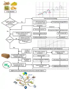
In policy analysis, forecasting future production of biofuels is key data for making better decisions, and statistical time series models have recently been developed to forecast renewable energy sources, and a multiplicative decomposition method was designed to forecast future production of biohydrogen. The optimum length of the moving average (seasonal length) and start point, where the averages are placed, were indicated based on the best coincidence between the present forecast and actual values.[5]

An example of statistical software for this type of decomposition is the program BV4.1 that is based on the Berlin procedure. The R statistical software also includes many packages for time series decomposition, such as seasonal,[7] stl, stlplus,[8] and bfast. Bayesian methods are also available; one example is the BEAST method in a package Rbeast [9] in R, Matlab, and Python.

• Frequency spectrum
• Hilbert–Huang transform
• Least squares
• Least-squares spectral analysis
• Stochastic drift
• Trend filtering

• Enders, Walter (2004). "Models with Trend". Applied Econometric Time Series (Second ed.). New York: Wiley. pp. 156–238. ISBN 0-471-23065-0.

References

- "6.1 Time series components | OTexts". www.otexts.org. Retrieved 2016-05-14.
- Dodge, Y. (2003). The Oxford Dictionary of Statistical Terms. New York: Oxford University Press. ISBN 0-19-920613-9.
- "6.1 Time series components | OTexts". www.otexts.org. Retrieved 2016-05-18.
- "6.5 STL decomposition | OTexts". www.otexts.org. Retrieved 2016-05-18.
- Asadi, Nooshin; Karimi Alavijeh, Masih; Zilouei, Hamid (2016). "Development of a mathematical methodology to investigate biohydrogen production from regional and national agricultural crop residues: A case study of Iran". International Journal of Hydrogen Energy. doi:10.1016/j.ijhydene.2016.10.021.
- Kendall, M. G. (1976). Time-Series (Second ed.). Charles Griffin. (Fig. 5.1). ISBN 0-85264-241-5.
- Sax, Christoph. "seasonal: R Interface to X-13-ARIMA-SEATS".
- Hafen, Ryan. "stlplus: Enhanced Seasonal Decomposition of Time Series by Loess".
- Li, Yang; Zhao, Kaiguang; Hu, Tongxi; Zhang, Xuesong. "BEAST: A Bayesian Ensemble Algorithm for Change-Point Detection and Time Series Decomposition".
Further reading