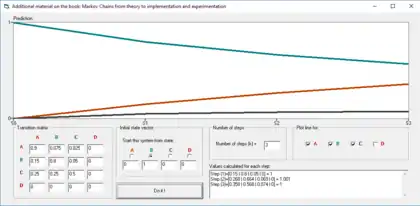
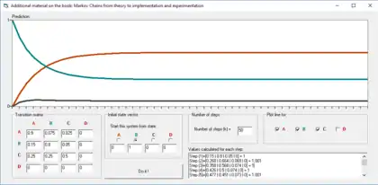
Examples of Markov chains

A game of snakes and ladders or any other game whose moves are determined entirely by dice is a Markov chain, indeed, an absorbing Markov chain. This is in contrast to card games such as blackjack, where the cards represent a 'memory' of the past moves. To see the difference, consider the probability for a certain event in the game. In the above-mentioned dice games, the only thing that matters is the current state of the board. The next state of the board depends on the current state, and the next roll of the dice. It doesn't depend on how things got to their current state. In a game such as blackjack, a player can gain an advantage by remembering which cards have already been shown (and hence which cards are no longer in the deck), so the next state (or hand) of the game is not independent of the past states.

Consider a random walk on the number line where, at each step, the position (call it x) may change by +1 (to the right) or −1 (to the left) with probabilities:

${\displaystyle P_{\mathrm {move~left} }={\dfrac {1}{2}}+{\dfrac {1}{2}}\left({\dfrac {x}{c+|x|}}\right)}$

${\displaystyle P_{\mathrm {move~right} }=1-P_{\mathrm {move~left} }}$

(where c is a constant greater than 0)

For example, if the constant, c, equals 1, the probabilities of a move to the left at positions x = −2,−1,0,1,2 are given by ${\displaystyle {\dfrac {1}{6}},{\dfrac {1}{4}},{\dfrac {1}{2}},{\dfrac {3}{4}},{\dfrac {5}{6}}}$ respectively. The random walk has a centering effect that weakens as c increases.

Since the probabilities depend only on the current position (value of x) and not on any prior positions, this biased random walk satisfies the definition of a Markov chain.

Suppose that you start with $10, and you wager $1 on an unending, fair, coin toss indefinitely, or until you lose all of your money. If ${\displaystyle X_{n}}$ represents the number of dollars you have after n tosses, with ${\displaystyle X_{0}=10}$, then the sequence ${\displaystyle \{X_{n}:n\in \mathbb {N} \}}$ is a Markov process. If I know that you have $12 now, then it would be expected that with even odds, you will either have $11 or $13 after the next toss. This guess is not improved by the added knowledge that you started with $10, then went up to $11, down to $10, up to $11, and then to $12. The fact that the guess is not improved by the knowledge of earlier tosses showcases the Markov property, the memoryless property of a stochastic process.[1][2]

The probabilities of weather conditions (modeled as either rainy or sunny), given the weather on the preceding day, can be represented by a transition matrix:[3]

${\displaystyle P={\begin{bmatrix}0.9&0.1\\0.5&0.5\end{bmatrix}}}$

The matrix P represents the weather model in which a sunny day is 90% likely to be followed by another sunny day, and a rainy day is 50% likely to be followed by another rainy day.[3] The columns can be labelled "sunny" and "rainy", and the rows can be labelled in the same order.

The above matrix as a graph.

(P)_{i j} is the probability that, if a given day is of type i, it will be followed by a day of type j.

Notice that the rows of P sum to 1: this is because P is a stochastic matrix.[3]

The weather on day 0 (today) is known to be sunny. This is represented by an initial state vector in which the "sunny" entry is 100%, and the "rainy" entry is 0%:

${\displaystyle \mathbf {x} ^{(0)}={\begin{bmatrix}1&0\end{bmatrix}}}$

The weather on day 1 (tomorrow) can be predicted by multiplying the state vector from day 0 by the transition matrix:

${\displaystyle \mathbf {x} ^{(1)}=\mathbf {x} ^{(0)}P={\begin{bmatrix}1&0\end{bmatrix}}{\begin{bmatrix}0.9&0.1\\0.5&0.5\end{bmatrix}}={\begin{bmatrix}0.9&0.1\end{bmatrix}}}$

Thus, there is a 90% chance that day 1 will also be sunny.

The weather on day 2 (the day after tomorrow) can be predicted in the same way, from the state vector we computed for day 1:

${\displaystyle \mathbf {x} ^{(2)}=\mathbf {x} ^{(1)}P=\mathbf {x} ^{(0)}P^{2}={\begin{bmatrix}1&0\end{bmatrix}}{\begin{bmatrix}0.9&0.1\\0.5&0.5\end{bmatrix}}^{2}={\begin{bmatrix}0.86&0.14\end{bmatrix}}}$

or

${\displaystyle \mathbf {x} ^{(2)}=\mathbf {x} ^{(1)}P={\begin{bmatrix}0.9&0.1\end{bmatrix}}{\begin{bmatrix}0.9&0.1\\0.5&0.5\end{bmatrix}}={\begin{bmatrix}0.86&0.14\end{bmatrix}}}$

General rules for day n are:

${\displaystyle \mathbf {x} ^{(n)}=\mathbf {x} ^{(n-1)}P}$

${\displaystyle \mathbf {x} ^{(n)}=\mathbf {x} ^{(0)}P^{n}}$

In this example, predictions for the weather on more distant days change less and less on each subsequent day and tend towards a steady state vector.[4] This vector represents the probabilities of sunny and rainy weather on all days, and is independent of the initial weather.[4]

The steady state vector is defined as:

${\displaystyle \mathbf {q} =\lim _{n\to \infty }\mathbf {x} ^{(n)}}$

but converges to a strictly positive vector only if P is a regular transition matrix (that is, there is at least one Pⁿ with all non-zero entries).

Since q is independent from initial conditions, it must be unchanged when transformed by P.[4] This makes it an eigenvector (with eigenvalue 1), and means it can be derived from P.[4]

In layman's terms, the steady-state vector is the vector that, when we multiply it by P, we get the exact same vector back.[5] For the weather example, we can use this to set up a matrix equation:

${\displaystyle {\begin{aligned}P&={\begin{bmatrix}0.9&0.1\\0.5&0.5\end{bmatrix}}\\\mathbf {q} P&=\mathbf {q} &&{\text{(}}\mathbf {q} {\text{ is unchanged by }}P{\text{.)}}\\&=\mathbf {q} I\\\mathbf {q} (P-I)&=\mathbf {0} \\\mathbf {q} \left({\begin{bmatrix}0.9&0.1\\0.5&0.5\end{bmatrix}}-{\begin{bmatrix}1&0\\0&1\end{bmatrix}}\right)&=\mathbf {0} \\\mathbf {q} {\begin{bmatrix}-0.1&0.1\\0.5&-0.5\end{bmatrix}}&=\mathbf {0} \\{\begin{bmatrix}q_{1}&q_{2}\end{bmatrix}}{\begin{bmatrix}-0.1&0.1\\0.5&-0.5\end{bmatrix}}&={\begin{bmatrix}0&0\end{bmatrix}}\\-0.1q_{1}+0.5q_{2}&=0\end{aligned}}}$

and since they are a probability vector we know that

${\displaystyle q_{1}+q_{2}=1.}$

Solving this pair of simultaneous equations gives the steady state vector:

${\displaystyle {\begin{bmatrix}q_{1}&q_{2}\end{bmatrix}}={\begin{bmatrix}0.833&0.167\end{bmatrix}}}$

In conclusion, in the long term about 83.3% of days are sunny. It is important to realize that not all Markov processes have a steady state vector. In particular, the transition matrix must be regular. Otherwise, the state vectors will oscillate over time without converging.

Using a directed graph, the probabilities of the possible states a hypothetical stock market can exhibit is represented. The matrix on the left shows how probabilities corresponding to different states can be arranged in matrix form.

A state diagram for a simple example is shown in the figure on the right, using a directed graph to picture the state transitions. The states represent whether a hypothetical stock market is exhibiting a bull market, bear market, or stagnant market trend during a given week. According to the figure, a bull week is followed by another bull week 90% of the time, a bear week 7.5% of the time, and a stagnant week the other 2.5% of the time. Labeling the state space {1 = bull, 2 = bear, 3 = stagnant} the transition matrix for this example is

${\displaystyle P={\begin{bmatrix}0.9&0.075&0.025\\0.15&0.8&0.05\\0.25&0.25&0.5\end{bmatrix}}.}$

The distribution over states can be written as a stochastic row vector x with the relation x^(n + 1) = x⁽ⁿ⁾P. So if at time n the system is in state x⁽ⁿ⁾, then three time periods later, at time n + 3 the distribution is

${\displaystyle {\begin{aligned}x^{(n+3)}&=x^{(n+2)}P=\left(x^{(n+1)}P\right)P\\\\&=x^{(n+1)}P^{2}=\left(x^{(n)}P\right)P^{2}\\&=x^{(n)}P^{3}\\\end{aligned}}}$

Markov Chains prediction on 3 discrete steps based on the transition matrix from the example to the left.[6]

In particular, if at time n the system is in state 2 (bear), then at time n + 3 the distribution is

${\displaystyle {\begin{aligned}x^{(n+3)}&={\begin{bmatrix}0&1&0\end{bmatrix}}{\begin{bmatrix}0.9&0.075&0.025\\0.15&0.8&0.05\\0.25&0.25&0.5\end{bmatrix}}^{3}\\[5pt]&={\begin{bmatrix}0&1&0\end{bmatrix}}{\begin{bmatrix}0.7745&0.17875&0.04675\\0.3575&0.56825&0.07425\\0.4675&0.37125&0.16125\\\end{bmatrix}}\\[5pt]&={\begin{bmatrix}0.3575&0.56825&0.07425\end{bmatrix}}.\end{aligned}}}$

Markov chains prediction on 50 discrete steps. Again, the transition matrix from the left is used.[6]

Using the transition matrix it is possible to calculate, for example, the long-term fraction of weeks during which the market is stagnant, or the average number of weeks it will take to go from a stagnant to a bull market. Using the transition probabilities, the steady-state probabilities indicate that 62.5% of weeks will be in a bull market, 31.25% of weeks will be in a bear market and 6.25% of weeks will be stagnant, since:

${\displaystyle \lim _{N\to \infty }\,P^{N}={\begin{bmatrix}0.625&0.3125&0.0625\\0.625&0.3125&0.0625\\0.625&0.3125&0.0625\end{bmatrix}}}$

A thorough development and many examples can be found in the on-line monograph Meyn & Tweedie 2005.[7]

A finite-state machine can be used as a representation of a Markov chain. Assuming a sequence of independent and identically distributed input signals (for example, symbols from a binary alphabet chosen by coin tosses), if the machine is in state y at time n, then the probability that it moves to state x at time n + 1 depends only on the current state.

If one pops one hundred kernels of popcorn in an oven, each kernel popping at an independent exponentially-distributed time, then this would be a continuous-time Markov process. If ${\displaystyle X_{t}}$ denotes the number of kernels which have popped up to time t, the problem can be defined as finding the number of kernels that will pop in some later time. The only thing one needs to know is the number of kernels that have popped prior to the time "t". It is not necessary to know when they popped, so knowing ${\displaystyle X_{t}}$ for previous times "t" is not relevant.

The process described here is an approximation of a Poisson point process – Poisson processes are also Markov processes.

References

- Øksendal, B. K. (Bernt Karsten), 1945- (2003). Stochastic differential equations : an introduction with applications (6th ed.). Berlin: Springer. ISBN 3540047581. OCLC 52203046.
{{cite book}}: CS1 maint: multiple names: authors list (link) - Gagniuc, Paul A. (2017). Markov Chains: From Theory to Implementation and Experimentation. USA, NJ: John Wiley & Sons. pp. 1–235. ISBN 978-1-119-38755-8.
- Van Kampen, N.G. (2007). Stochastic Processes in Physics and Chemistry. NL: North Holland Elsevier. pp. 73–95. ISBN 978-0-444-52965-7.
- "Going steady (state) with Markov processes". Bloomington Tutors.
- Gagniuc, Paul A. (2017). Markov chains: from theory to implementation and experimentation. Hoboken, NJ: John Wiley & Sons. pp. 131–163. ISBN 9781119387572. OCLC 982373850.
- S. P. Meyn and R.L. Tweedie, 2005. Markov Chains and Stochastic Stability Archived 2013-09-03 at the Wayback Machine