Factorial experiment
In statistics, a full factorial experiment is an experiment whose design consists of two or more factors, each with discrete possible values or "levels", and whose experimental units take on all possible combinations of these levels across all such factors. A full factorial design may also be called a fully crossed design. Such an experiment allows the investigator to study the effect of each factor on the response variable, as well as the effects of interactions between factors on the response variable.
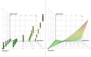
For the vast majority of factorial experiments, each factor has only two levels. For example, with two factors each taking two levels, a factorial experiment would have four treatment combinations in total, and is usually called a 2×2 factorial design. In such a design, the interaction between the variables is often the most important. This applies even to scenarios where a main effect and an interaction are present.
If the number of combinations in a full factorial design is too high to be logistically feasible, a fractional factorial design may be done, in which some of the possible combinations (usually at least half) are omitted.
Other terms for "treatment combinations" are often used, such as runs (of an experiment), points (viewing the combinations as vertices of a graph, and cells (arising as intersections of rows and columns).
History
Factorial designs were used in the 19th century by John Bennet Lawes and Joseph Henry Gilbert of the Rothamsted Experimental Station.[1]
Ronald Fisher argued in 1926 that "complex" designs (such as factorial designs) were more efficient than studying one factor at a time.[2] Fisher wrote,
"No aphorism is more frequently repeated in connection with field trials, than that we must ask Nature few questions, or, ideally, one question, at a time. The writer is convinced that this view is wholly mistaken."
Nature, he suggests, will best respond to "a logical and carefully thought out questionnaire". A factorial design allows the effect of several factors and even interactions between them to be determined with the same number of trials as are necessary to determine any one of the effects by itself with the same degree of accuracy.
Frank Yates made significant contributions, particularly in the analysis of designs, by the Yates analysis.
The term "factorial" may not have been used in print before 1935, when Fisher used it in his book The Design of Experiments.[3]
Advantages and disadvantages of factorial experiments
Many people examine the effect of only a single factor or variable. Compared to such one-factor-at-a-time (OFAT) experiments, factorial experiments offer several advantages[4][5]
- Factorial designs are more efficient than OFAT experiments. They provide more information at similar or lower cost. They can find optimal conditions faster than OFAT experiments.
- When the effect of one factor is different for different levels of another factor, it cannot be detected by an OFAT experiment design. Factorial designs are required to detect such interactions. Use of OFAT when interactions are present can lead to serious misunderstanding of how the response changes with the factors.
- Factorial designs allow the effects of a factor to be estimated at several levels of the other factors, yielding conclusions that are valid over a range of experimental conditions.
The main disadvantage of the full factorial design is its sample size requirement, which grows exponentially with the number of factors or inputs considered.[6] Alternative strategies with improved computational efficiency include fractional factorial designs, Latin hypercube sampling, and quasi-random sampling techniques.
Example of advantages of factorial experiments
In his book, Improving Almost Anything: Ideas and Essays, statistician George Box gives many examples of the benefits of factorial experiments. Here is one.[7] Engineers at the bearing manufacturer SKF wanted to know if changing to a less expensive "cage" design would affect bearing life. The engineers asked Christer Hellstrand, a statistician, for help in designing the experiment.[8]
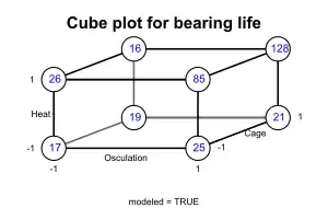
Box reports the following. "The results were assessed by an accelerated life test. … The runs were expensive because they needed to be made on an actual production line and the experimenters were planning to make four runs with the standard cage and four with the modified cage. Christer asked if there were other factors they would like to test. They said there were, but that making added runs would exceed their budget. Christer showed them how they could test two additional factors "for free" – without increasing the number of runs and without reducing the accuracy of their estimate of the cage effect. In this arrangement, called a 2×2×2 factorial design, each of the three factors would be run at two levels and all the eight possible combinations included. The various combinations can conveniently be shown as the vertices of a cube ... " "In each case, the standard condition is indicated by a minus sign and the modified condition by a plus sign. The factors changed were heat treatment, outer ring osculation, and cage design. The numbers show the relative lengths of lives of the bearings. If you look at [the cube plot], you can see that the choice of cage design did not make a lot of difference. … But, if you average the pairs of numbers for cage design, you get the [table below], which shows what the two other factors did. … It led to the extraordinary discovery that, in this particular application, the life of a bearing can be increased fivefold if the two factor(s) outer ring osculation and inner ring heat treatments are increased together."
| Osculation − | Osculation + | |
|---|---|---|
| Heat − | 18 | 23 |
| Heat + | 21 | 106 |
"Remembering that bearings like this one have been made for decades, it is at first surprising that it could take so long to discover so important an improvement. A likely explanation is that, because most engineers have, until recently, employed only one factor at a time experimentation, interaction effects have been missed."
Example
The simplest factorial experiment contains two levels for each of two factors. Suppose an engineer wishes to study the total power used by each of two different motors, A and B, running at each of two different speeds, 2000 or 3000 RPM. The factorial experiment would consist of four experimental units: motor A at 2000 RPM, motor B at 2000 RPM, motor A at 3000 RPM, and motor B at 3000 RPM. Each combination of a single level selected from every factor is present once.
This experiment is an example of a 22 (or 2×2) factorial experiment, so named because it considers two levels (the base) for each of two factors (the power or superscript), or #levels#factors, producing 22=4 factorial points.
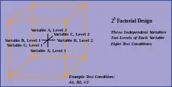
Designs can involve many independent variables. As a further example, the effects of three input variables can be evaluated in eight experimental conditions shown as the corners of a cube.
This can be conducted with or without replication, depending on its intended purpose and available resources. It will provide the effects of the three independent variables on the dependent variable and possible interactions.
Notation
| A | B | |
|---|---|---|
| (1) | − | − |
| a | + | − |
| b | − | + |
| ab | + | + |
The notation used to denote factorial experiments conveys a lot of information. When a design is denoted a 23 factorial, this identifies the number of factors (3); how many levels each factor has (2); and how many experimental conditions there are in the design (23 = 8). Similarly, a 25 design has five factors, each with two levels, and 25 = 32 experimental conditions. Factorial experiments can involve factors with different numbers of levels. A 243 design has five factors, four with two levels and one with three levels, and has 16 × 3 = 48 experimental conditions. [9]
To save space, the points in a two-level factorial experiment are often abbreviated with strings of plus and minus signs. The strings have as many symbols as factors, and their values dictate the level of each factor: conventionally, for the first (or low) level, and for the second (or high) level. The points in this experiment can thus be represented as , , , and . Another common and useful notation for the two levels is 0 and 1, so that the treatment combinations are 00, 01, 10, and 11.
The factorial points can also be abbreviated by (1), a, b, and ab, where the presence of a letter indicates that the specified factor is at its high (or second) level and the absence of a letter indicates that the specified factor is at its low (or first) level (for example, "a" indicates that factor A is on its high setting, while all other factors are at their low (or first) setting). (1) is used to indicate that all factors are at their lowest (or first) values.
In an (or ) factorial experiment, there are k factors, the ith factor at levels. If is the set of levels of the ith factor, then the set of treatment combinations is the Cartesian product . A treatment combination is thus a k-tuple . If , say, the experiment is said to be symmetric and of type , and the same set is used to denote the set of levels of each factor. In a 2-level experiment, for example, one may take , as above; the treatment combination is by denoted (1), by a, and so on.
Implementation
For more than two factors, a 2k factorial experiment can usually be recursively designed from a 2k−1 factorial experiment by replicating the 2k−1 experiment, assigning the first replicate to the first (or low) level of the new factor, and the second replicate to the second (or high) level. This framework can be generalized to, e.g., designing three replicates for three level factors, etc.
A factorial experiment allows for estimation of experimental error in two ways. The experiment can be replicated, or the sparsity-of-effects principle can often be exploited. Replication is more common for small experiments and is a very reliable way of assessing experimental error. When the number of factors is large (typically more than about 5 factors, but this does vary by application), replication of the design can become operationally difficult. In these cases, it is common to only run a single replicate of the design, and to assume that factor interactions of more than a certain order (say, between three or more factors) are negligible. Under this assumption, estimates of such high order interactions are estimates of an exact zero, thus really an estimate of experimental error.
When there are many factors, many experimental runs will be necessary, even without replication. For example, experimenting with 10 factors at two levels each produces 210=1024 combinations. At some point this becomes infeasible due to high cost or insufficient resources. In this case, fractional factorial designs may be used.
As with any statistical experiment, the experimental runs in a factorial experiment should be randomized to reduce the impact that bias could have on the experimental results. In practice, this can be a large operational challenge.
Factorial experiments can be used when there are more than two levels of each factor. However, the number of experimental runs required for three-level (or more) factorial designs will be considerably greater than for their two-level counterparts. Factorial designs are therefore less attractive if a researcher wishes to consider more than two levels.
Main effects and interactions
A fundamental concept in experimental design is the contrast. Let be the expected response to treatment combination , and let be the set of treatment combinations. A contrast in is a linear expression such that . The function is a contrast function. Typically the order of the treatment combinations t is fixed, so that is a contrast vector with components . These vectors will be written as columns.
- Example: In a one-factor experiment the expression represents a contrast between level 1 of the factor and the combined impact of levels 2 and 3. The corresponding contrast function is given by , and the contrast vector is , the transpose (T) indicating a column.
Contrast vectors belong to the Euclidean space , where , the number of treatment combinations. It is easy to see that if and are contrast vectors, so is , and so is for any real number . As usual, contrast vectors and are said to be orthogonal (denoted ) if their dot product is zero, that is, if .
More generally, Bose[10] has given the following definitions:
- A contrast vector belongs to the main effect of factor i if the value of depends only on .
- Example: In the illustration above, the contrast represents the main effect of factor , as the coefficients in this expression depend only on the level of (high versus low). The contrast vector is displayed in the column for factor in the table above. Any scalar multiple of this vector also belongs to this main effect. For example, it is common to put the factor 1/2 in front of the contrast describing a main effect in a experiment, so that the contrast for compares two averages rather than two sums.
- The contrast vector belongs to the interaction between factors i and j if (a) the value of depends only on and , and (b) is orthogonal to the contrast vectors for the main effects of factors and .
- These contrasts detect the presence or absence of additivity between the two factors.[11][12] Additivity may be viewed as a kind of parallelism between factors, as illustrated in the Analysis section below. Interaction is lack of additivity.
- Example: In the experiment above, additivity is expressed by the equality , which can be written . In the latter equation, the expression on the left-hand side is a contrast, and the corresponding contrast vector would be . It is orthogonal to the contrast vectors for and . Any scalar multiple of this vector also belongs to interaction.
- Similarly, for any subset of having more than two elements, a contrast vector belongs the interaction between the factors listed in if (a) the value of depends only on the levels and (b) is orthogonal to all contrasts of lower order among those factors.
Let denote the set of contrast vectors belonging to the main effect of factor , the set of those belonging to the interaction between factors and , and more generally the set of contrast vectors belonging to the interaction between the factors listed in for any subset with (here again denotes cardinality). In addition, let denote the set of constant vectors on , that is, vectors whose components are equal. This defines a set corresponding to each . It is not hard to see that each is a vector space, a subspace of , where (as before) , the number of treatment combinations. The following are well-known, fundamental facts:[13][14]
- If then .
- is the sum of all the subspaces .
- For each , dim . (The empty product is defined to be 1.)
These results underpin the usual analysis of variance or ANOVA (see below), in which a total sum of squares is partitioned into the sums of squares for each effect (main effect or interaction), as introduced by Fisher. The dimension of is the degrees of freedom for the corresponding effect.
- Example: In a two-factor or experiment the orthogonal sum reads
- ,
- and the corresponding dimensions are
- ,
- giving the usual formulas for degrees of freedom for main effects and interaction (the total degrees of freedom is ).
The next section illustrates these ideas in a experiment.
Components of interaction and confounding with blocks
In certain symmetric factorial experiments the sets that represent interactions can themselves be decomposed orthogonally. A key application, confounding with blocks, is described at the end of this section.
Consider the following example in which each of two factors, and , has 3 levels, denoted 0, 1 and 2. According to the formula in the previous section, such an experiment has 2 degrees of freedom for each main effect and 4 for interaction (that is, and ).
The layout table below on the left describes the nine cells or treatment combinations , which are written without parentheses or commas (for example, (1,2) is written 12).
In the contrasts table at right, the first column lists these cells, while the last eight columns contain contrast vectors. The columns labeled and belong to the main effects of those two factors, as explained below. The last four columns are orthogonal to both and so must belong to interaction. (In fact, these eight vectors are bases of , , and , respectively.) In addition, the last four columns have been separated into two sets of two. These two effects, which are usually labelled and , are components of interaction, each having 2 degrees of freedom.
| 0 | 1 | 2 | |
| 0 | 00 | 01 | 02 |
| 1 | 10 | 11 | 12 |
| 2 | 20 | 21 | 22 |
| cell | ||||||||||
|---|---|---|---|---|---|---|---|---|---|---|
| 00 | 0 | 0 | 1 | 1 | 1 | 1 | 1 | 1 | 1 | 1 |
| 01 | 1 | 2 | 1 | 1 | -1 | 0 | -1 | 0 | 0 | -1 |
| 02 | 2 | 1 | 1 | 1 | 0 | -1 | 0 | -1 | -1 | 0 |
| 10 | 1 | 1 | -1 | 0 | 1 | 1 | -1 | 0 | -1 | 0 |
| 11 | 2 | 0 | -1 | 0 | -1 | 0 | 0 | -1 | 1 | 1 |
| 12 | 0 | 2 | -1 | 0 | 0 | -1 | 1 | 1 | 0 | -1 |
| 20 | 2 | 2 | 0 | -1 | 1 | 1 | 0 | -1 | 0 | -1 |
| 21 | 0 | 1 | 0 | -1 | -1 | 0 | 1 | 1 | -1 | 0 |
| 22 | 1 | 0 | 0 | -1 | 0 | -1 | -1 | 0 | 1 | 1 |
It is easy to see that the contrast vectors labeled depend only on the values of (the first component of each cell), so that these vectors indeed belong to the main effect of . Similarly, those labeled belong to that main effect since they depend only on the values of ; sorting the column and comparing with the column of cells makes this easier to see.
In a similar fashion, the and contrast vectors depend respectively on the values of and modulo 3, which are contained in the second and third columns of the table. To see this easily, one may sort the contrasts table by the value of and observe how the values of the contrast vectors follow the same pattern as those of . The same holds for and .
One can verify that the contrast vectors of are orthogonal to those of . One should also note this important naming convention: The exponents of and in the expressions and are the coefficients of and in the defining expressions and .
A key point is that each main effect and each component of interaction corresponds to a partition of the nine treatment combinations in three sets of three. The partitions for and are given respectively by the rows and columns of the layout table. To see the partitions corresponding to and , one may fill the layout table with the values of , and again with the values of :
| 0 | 1 | 2 |
| 1 | 2 | 0 |
| 2 | 0 | 1 |
| 0 | 2 | 1 |
| 1 | 0 | 2 |
| 2 | 1 | 0 |
In each table, the three cells labeled 0 form one block of a partition, and those labeled 1 and 2 form two other blocks.
(One may note in passing that each table is a Latin square of order 3. The two squares would in fact be mutually orthogonal. This orthogonality is what makes the contrast vectors perpendicular to those of , while latinity makes these vectors perpendicular to those of and .)
A similar result holds for any factorial experiment, or indeed any (= ) experiment, as long as the number is a prime (as in the above example) or a prime power (for example, or ).[15] Each component of interaction is defined by solving an equation
for , where the solution sets as varies form a partition of the treatment combinations. The necessary arithmetic is that of the finite field , which is simply arithmetic modulo when is prime. The same naming convention holds as in the example above: The component defined by the expression is labeled . Every interaction is then an orthogonal sum of components, each carrying degrees of freedom. Each component would then appear in the ANOVA table for such an experiment. Examples of such analyses can be found in some introductory texts.[16][17]
The fact that every component of interaction is defined by a partition (blocking) of the set of treatment combinations makes components of interaction the essential tool in dealing with factorial experiments that must be run in blocks, where certain effects will be confounded with blocks[18][19] (their contrasts will be identical to contrasts between blocks). Here the goal is to choose the blocking so as not to confound main effects and low-order interactions. For example, if it is necessary to run a experiment in 3 blocks of 3, one might choose the blocks defined by the component. This would confound with blocks, but would leave the main effects and the component unconfounded.
Analysis
A factorial experiment can be analyzed using ANOVA or regression analysis.[20] To compute the main effect of a factor "A" in a 2-level experiment, subtract the average response of all experimental runs for which A was at its low (or first) level from the average response of all experimental runs for which A was at its high (or second) level.
Other useful exploratory analysis tools for factorial experiments include main effects plots, interaction plots, Pareto plots, and a normal probability plot of the estimated effects.
When the factors are continuous, two-level factorial designs assume that the effects are linear. If a quadratic effect is expected for a factor, a more complicated experiment should be used, such as a central composite design. Optimization of factors that could have quadratic effects is the primary goal of response surface methodology.
Analysis example
Montgomery[4] gives the following example of analysis of a factorial experiment:.
An engineer would like to increase the filtration rate (output) of a process to produce a chemical, and to reduce the amount of formaldehyde used in the process. Previous attempts to reduce the formaldehyde have lowered the filtration rate. The current filtration rate is 75 gallons per hour. Four factors are considered: temperature (A), pressure (B), formaldehyde concentration (C), and stirring rate (D). Each of the four factors will be tested at two levels.
Onwards, the minus (−) and plus (+) signs will indicate whether the factor is run at a low or high level, respectively.
| A | B | C | D | Filtration rate |
|---|---|---|---|---|
| − | − | − | − | 45 |
| + | − | − | − | 71 |
| − | + | − | − | 48 |
| + | + | − | − | 65 |
| − | − | + | − | 68 |
| + | − | + | − | 60 |
| − | + | + | − | 80 |
| + | + | + | − | 65 |
| − | − | − | + | 43 |
| + | − | − | + | 100 |
| − | + | − | + | 45 |
| + | + | − | + | 104 |
| − | − | + | + | 75 |
| + | − | + | + | 86 |
| − | + | + | + | 70 |
| + | + | + | + | 96 |
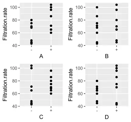 Plot of the main effects showing the filtration rates for the low (−) and high (+) settings for each factor.
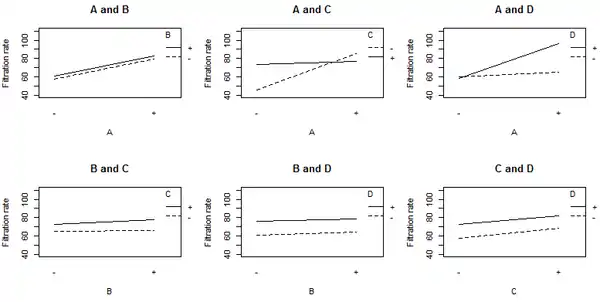 Plot of the interaction effects showing the mean filtration rate at each of the four possible combinations of levels for a given pair of factors.
The non-parallel lines in the A:C interaction plot indicate that the effect of factor A depends on the level of factor C. A similar results holds for the A:D interaction. The graphs indicate that factor B has little effect on filtration rate. The analysis of variance (ANOVA) including all 4 factors and all possible interaction terms between them yields the coefficient estimates shown in the table below.
| Coefficients | Estimate |
|---|---|
| Intercept | 70.063 |
| A | 10.813 |
| B | 1.563 |
| C | 4.938 |
| D | 7.313 |
| A:B | 0.063 |
| A:C | −9.063 |
| B:C | 1.188 |
| A:D | 8.313 |
| B:D | −0.188 |
| C:D | −0.563 |
| A:B:C | 0.938 |
| A:B:D | 2.063 |
| A:C:D | −0.813 |
| B:C:D | −1.313 |
| A:B:C:D | 0.688 |
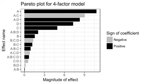
Because there are 16 observations and 16 coefficients (intercept, main effects, and interactions), p-values cannot be calculated for this model. The coefficient values and the graphs suggest that the important factors are A, C, and D, and the interaction terms A:C and A:D.
The coefficients for A, C, and D are all positive in the ANOVA, which would suggest running the process with all three variables set to the high value. However, the main effect of each variable is the average over the levels of the other variables. The A:C interaction plot above shows that the effect of factor A depends on the level of factor C, and vice versa. Factor A (temperature) has very little effect on filtration rate when factor C is at the + level. But Factor A has a large effect on filtration rate when factor C (formaldehyde) is at the − level. The combination of A at the + level and C at the − level gives the highest filtration rate. This observation indicates how one-factor-at-a-time analyses can miss important interactions. Only by varying both factors A and C at the same time could the engineer discover that the effect of factor A depends on the level of factor C.
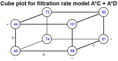
The best filtration rate is seen when A and D are at the high level, and C is at the low level. This result also satisfies the objective of reducing formaldehyde (factor C). Because B does not appear to be important, it can be dropped from the model. Performing the ANOVA using factors A, C, and D, and the interaction terms A:C and A:D, gives the result shown in the following table, in which all the terms are significant (p-value < 0.05).
| Coefficient | Estimate | Standard error | t value | p-value |
|---|---|---|---|---|
| Intercept | 70.062 | 1.104 | 63.444 | 2.3 × 10⁻¹⁴ |
| A | 10.812 | 1.104 | 9.791 | 1.9 × 10⁻⁶ |
| C | 4.938 | 1.104 | 4.471 | 1.2 × 10⁻³ |
| D | 7.313 | 1.104 | 6.622 | 5.9 × 10⁻⁵ |
| A:C | −9.063 | 1.104 | −8.206 | 9.4 × 10⁻⁶ |
| A:D | 8.312 | 1.104 | 7.527 | 2 × 10⁻⁵ |
See also
Notes
- Yates, Frank; Mather, Kenneth (1963). "Ronald Aylmer Fisher". Biographical Memoirs of Fellows of the Royal Society. London, England: Royal Society. 9: 91–120. doi:10.1098/rsbm.1963.0006.
- Fisher, Ronald (1926). "The Arrangement of Field Experiments" (PDF). Journal of the Ministry of Agriculture of Great Britain. London, England: Ministry of Agriculture and Fisheries. 33: 503–513.
- "Earliest Known Uses of Some of the Words of Mathematics (F)". jeff560.tripod.com.
- Montgomery, Douglas C. (2013). Design and Analysis of Experiments (8th ed.). Hoboken, New Jersey: Wiley. ISBN 978-1-119-32093-7.
- Oehlert, Gary (2000). A First Course in Design and Analysis of Experiments (Revised ed.). New York City: W. H. Freeman and Company. ISBN 978-0-7167-3510-6.
- Tong, C. (2006). "Refinement strategies for stratified sampling methods". Reliability Engineering & System Safety. 91 (10–11): 1257–1265.
- George E.P., Box (2006). Improving Almost Anything: Ideas and Essays (Revised ed.). Hoboken, New Jersey: Wiley. ASIN B01FKSM9VY.
- Hellstrand, C.; Oosterhoorn, A. D.; Sherwin, D. J.; Gerson, M. (24 February 1989). "The Necessity of Modern Quality Improvement and Some Experience with its Implementation in the Manufacture of Rolling Bearings [and Discussion]". Philosophical Transactions of the Royal Society. 327 (1596): 529–537. doi:10.1098/rsta.1989.0008. S2CID 122252479.
- Penn State University College of Health and Human Development (2011-12-22). "Introduction to Factorial Experimental Designs".
- Bose (1947, pp. 110–111)
- Beder (2022, pp. 29–30)
- Graybill (1976, pp. 559–560)
- Beder (2022, pp. 164–165)
- Cheng (2019, pp. 77–81)
- Beder (2022, pp. 180-190, 193-195)
- Hicks (1982, p. 298)
- Wu & Hamada (2021, p. 269)
- Dean, Voss & Draguljić (2017, Sec. 14.2)
- Montgomery (2013, Confounding in the Factorial Design; Confounding in the Factorial Design)
- Cohen, J (1968). "Multiple regression as a general data-analytic system". Psychological Bulletin. 70 (6): 426–443. CiteSeerX 10.1.1.476.6180. doi:10.1037/h0026714.
References
- Beder, Jay H. (2022). Linear Models and Design. Cham, Switzerland: Springer. doi:10.1007/978-3-031-08176-7. ISBN 978-3-031-08175-0. S2CID 253542415.
- Bose, R. C. (1947). "Mathematical theory of the symmetrical factorial design". Sankhya. 8: 107–166.
- Box, G. E.; Hunter, W. G.; Hunter, J. S. (2005). Statistics for Experimenters: Design, Innovation, and Discovery (2nd ed.). Wiley. ISBN 978-0-471-71813-0.
- Cheng, Ching-Shui (2019). Theory of Factorial Design: Single- and Multi-Stratum Experiments. Boca Raton, Florida: CRC Press. ISBN 978-0-367-37898-1.
- Dean, Angela; Voss, Daniel; Draguljić, Danel (2017). Design and Analysis of Experiments (2nd ed.). Cham, Switzerland: Springer. ISBN 978-3-319-52250-0.
- Graybill, Franklin A. (1976). Fundamental Concepts in the Design of Experiments (3rd ed.). New York: Holt, Rinehart and Winston. ISBN 0-03-061706-5.
- Hicks, Charles R. (1982). Theory and Application of the Linear Model. Pacific Grove, CA: Wadsworth & Brooks/Cole. ISBN 0-87872-108-8.
- Wu, C. F. Jeff; Hamada, Michael S. (30 March 2021). Experiments: Planning, Analysis, and Optimization. John Wiley & Sons. ISBN 978-1-119-47010-6.