Goldfeld–Quandt test
In statistics, the Goldfeld–Quandt test checks for homoscedasticity in regression analyses. It does this by dividing a dataset into two parts or groups, and hence the test is sometimes called a two-group test. The Goldfeld–Quandt test is one of two tests proposed in a 1965 paper by Stephen Goldfeld and Richard Quandt. Both a parametric and nonparametric test are described in the paper, but the term "Goldfeld–Quandt test" is usually associated only with the former.

Test

In the context of multiple regression (or univariate regression), the hypothesis to be tested is that the variances of the errors of the regression model are not constant, but instead are monotonically related to a pre-identified explanatory variable. For example, data on income and consumption may be gathered and consumption regressed against income. If the variance increases as levels of income increase, then income may be used as an explanatory variable. Otherwise some third variable (e.g. wealth or last period income) may be chosen.[1]
Parametric test
The parametric test is accomplished by undertaking separate least squares analyses on two subsets of the original dataset: these subsets are specified so that the observations for which the pre-identified explanatory variable takes the lowest values are in one subset, with higher values in the other. The subsets needs not be of equal size, nor contain all the observations between them. The parametric test assumes that the errors have a normal distribution. There is an additional assumption here, that the design matrices for the two subsets of data are both of full rank. The test statistic used is the ratio of the mean square residual errors for the regressions on the two subsets. This test statistic corresponds to an F-test of equality of variances, and a one- or two-sided test may be appropriate depending on whether or not the direction of the supposed relation of the error variance to the explanatory variable is known.[2]
Increasing the number of observations dropped in the "middle" of the ordering will increase the power of the test but reduce the degrees of freedom for the test statistic. As a result of this tradeoff it is common to see the Goldfeld–Quandt test performed by dropping the middle third of observations with smaller proportions of dropped observations as sample size increases.[3][4]
Nonparametric test
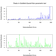
The second test proposed in the paper is a nonparametric one and hence does not rely on the assumption that the errors have a normal distribution. For this test, a single regression model is fitted to the complete dataset. The squares of the residuals are listed according to the order of the pre-identified explanatory variable. The test statistic used to test for homogeneity is the number of peaks in this list: ie. the count of the number of cases in which a squared residual is larger than all previous squared residuals.[5] Critical values for this test statistic are constructed by an argument related to permutation tests.
Advantages and disadvantages
The parametric Goldfeld–Quandt test offers a simple and intuitive diagnostic for heteroskedastic errors in a univariate or multivariate regression model. However some disadvantages arise under certain specifications or in comparison to other diagnostics, namely the Breusch–Pagan test, as the Goldfeld–Quandt test is somewhat of an ad hoc test.[6] Primarily, the Goldfeld–Quandt test requires that data be ordered along a known explanatory variable. The parametric test orders along this explanatory variable from lowest to highest. If the error structure depends on an unknown variable or an unobserved variable the Goldfeld–Quandt test provides little guidance. Also, error variance must be a monotonic function of the specified explanatory variable. For example, when faced with a quadratic function mapping the explanatory variable to error variance the Goldfeld–Quandt test may improperly accept the null hypothesis of homoskedastic errors.
Robustness
Unfortunately the Goldfeld–Quandt test is not very robust to specification errors.[7] The Goldfeld–Quandt test detects non-homoskedastic errors but cannot distinguish between heteroskedastic error structure and an underlying specification problem such as an incorrect functional form or an omitted variable.[7] Jerry Thursby proposed a modification of the Goldfeld–Quandt test using a variation of the Ramsey RESET test in order to provide some measure of robustness.[7]
Small sample properties
Herbert Glejser, in his 1969 paper outlining the Glejser test, provides a small sampling experiment to test the power and sensitivity of the Goldfeld–Quandt test. His results show limited success for the Goldfeld–Quandt test except under cases of "pure heteroskedasticity"—where variance can be described as a function of only the underlying explanatory variable.[8]
Software implementations
Notes
- Goldfeld, Stephen M.; Quandt, R. E. (June 1965). "Some Tests for Homoscedasticity". Journal of the American Statistical Association. 60 (310): 539–547. doi:10.1080/01621459.1965.10480811. JSTOR 2282689.
- Kennedy, Peter (2008). A Guide to Econometrics (6th ed.). Blackwell. p. 116. ISBN 978-1-4051-8257-7.
- Kennedy (2008), p. 124
- Ruud, Paul A. (2000). An Introduction to Classical Econometric Theory. Oxford University Press. p. 424. ISBN 0-19-511164-8.
- Goldfeld & Quandt (1965), p. 542
- Cook, R. Dennis; Weisberg, S. (April 1983). "Diagnostics for heteroscedasticitiy in regression". Biometrika. 70 (1): 1–10. doi:10.1093/biomet/70.1.1. hdl:11299/199411. JSTOR 2335938.
- Thursby, Jerry (May 1982). "Misspecification, Heteroscedasticity, and the Chow and Goldfeld-Quandt Tests". The Review of Economics and Statistics. 64 (2): 314–321. doi:10.2307/1924311. JSTOR 1924311.
- Glejser, H. (March 1969). "A New Test for Heteroskedasticity". Journal of the American Statistical Association. 64 (325): 316–323. doi:10.1080/01621459.1969.10500976. JSTOR 2283741.
- "lmtest: Testing Linear Regression Models". CRAN.
- Kleiber, Christian; Zeileis, Achim (2008). Applied Econometrics with R. New York: Springer. pp. 102–103. ISBN 978-0-387-77316-2.
- "skedastic: Heteroskedasticity Diagnostics for Linear Regression Models". CRAN.