Levenberg–Marquardt algorithm

In mathematics and computing, the Levenberg–Marquardt algorithm (LMA or just LM), also known as the damped least-squares (DLS) method, is used to solve non-linear least squares problems. These minimization problems arise especially in least squares curve fitting. The LMA interpolates between the Gauss–Newton algorithm (GNA) and the method of gradient descent. The LMA is more robust than the GNA, which means that in many cases it finds a solution even if it starts very far off the final minimum. For well-behaved functions and reasonable starting parameters, the LMA tends to be slower than the GNA. LMA can also be viewed as Gauss–Newton using a trust region approach.

The algorithm was first published in 1944 by Kenneth Levenberg,[1] while working at the Frankford Army Arsenal. It was rediscovered in 1963 by Donald Marquardt,[2] who worked as a statistician at DuPont, and independently by Girard,[3] Wynne[4] and Morrison.[5]

The LMA is used in many software applications for solving generic curve-fitting problems. By using the Gauss–Newton algorithm it often converges faster than first-order methods.[6] However, like other iterative optimization algorithms, the LMA finds only a local minimum, which is not necessarily the global minimum.

The problem

The primary application of the Levenberg–Marquardt algorithm is in the least-squares curve fitting problem: given a set of $m$ empirical pairs $\left(x_{i},y_{i}\right)$ of independent and dependent variables, find the parameters ${\boldsymbol {\beta }}$ of the model curve $f\left(x,{\boldsymbol {\beta }}\right)$ so that the sum of the squares of the deviations $S\left({\boldsymbol {\beta }}\right)$ is minimized:

{\hat {\boldsymbol {\beta }}}\in \operatorname {argmin} \limits _{\boldsymbol {\beta }}S\left({\boldsymbol {\beta }}\right)\equiv \operatorname {argmin} \limits _{\boldsymbol {\beta }}\sum _{i=1}^{m}\left[y_{i}-f\left(x_{i},{\boldsymbol {\beta }}\right)\right]^{2},

which is assumed to be non-empty.

The solution

Like other numeric minimization algorithms, the Levenberg–Marquardt algorithm is an iterative procedure. To start a minimization, the user has to provide an initial guess for the parameter vector ${\boldsymbol {\beta }}$ . In cases with only one minimum, an uninformed standard guess like ${\boldsymbol {\beta }}^{\text{T}}={\begin{pmatrix}1,\ 1,\ \dots ,\ 1\end{pmatrix}}$ will work fine; in cases with multiple minima, the algorithm converges to the global minimum only if the initial guess is already somewhat close to the final solution.

In each iteration step, the parameter vector ${\boldsymbol {\beta }}$ is replaced by a new estimate ${\boldsymbol {\beta }}+{\boldsymbol {\delta }}$ . To determine ${\boldsymbol {\delta }}$ , the function $f\left(x_{i},{\boldsymbol {\beta }}+{\boldsymbol {\delta }}\right)$ is approximated by its linearization:

f\left(x_{i},{\boldsymbol {\beta }}+{\boldsymbol {\delta }}\right)\approx f\left(x_{i},{\boldsymbol {\beta }}\right)+\mathbf {J} _{i}{\boldsymbol {\delta }},

where

\mathbf {J} _{i}={\frac {\partial f\left(x_{i},{\boldsymbol {\beta }}\right)}{\partial {\boldsymbol {\beta }}}}

is the gradient (row-vector in this case) of $f$ with respect to ${\boldsymbol {\beta }}$ .

The sum $S\left({\boldsymbol {\beta }}\right)$ of square deviations has its minimum at a zero gradient with respect to ${\boldsymbol {\beta }}$ . The above first-order approximation of $f\left(x_{i},{\boldsymbol {\beta }}+{\boldsymbol {\delta }}\right)$ gives

S\left({\boldsymbol {\beta }}+{\boldsymbol {\delta }}\right)\approx \sum _{i=1}^{m}\left[y_{i}-f\left(x_{i},{\boldsymbol {\beta }}\right)-\mathbf {J} _{i}{\boldsymbol {\delta }}\right]^{2},

or in vector notation,

{\begin{aligned}S\left({\boldsymbol {\beta }}+{\boldsymbol {\delta }}\right)&\approx \left\|\mathbf {y} -\mathbf {f} \left({\boldsymbol {\beta }}\right)-\mathbf {J} {\boldsymbol {\delta }}\right\|^{2}\\&=\left[\mathbf {y} -\mathbf {f} \left({\boldsymbol {\beta }}\right)-\mathbf {J} {\boldsymbol {\delta }}\right]^{\mathrm {T} }\left[\mathbf {y} -\mathbf {f} \left({\boldsymbol {\beta }}\right)-\mathbf {J} {\boldsymbol {\delta }}\right]\\&=\left[\mathbf {y} -\mathbf {f} \left({\boldsymbol {\beta }}\right)\right]^{\mathrm {T} }\left[\mathbf {y} -\mathbf {f} \left({\boldsymbol {\beta }}\right)\right]-\left[\mathbf {y} -\mathbf {f} \left({\boldsymbol {\beta }}\right)\right]^{\mathrm {T} }\mathbf {J} {\boldsymbol {\delta }}-\left(\mathbf {J} {\boldsymbol {\delta }}\right)^{\mathrm {T} }\left[\mathbf {y} -\mathbf {f} \left({\boldsymbol {\beta }}\right)\right]+{\boldsymbol {\delta }}^{\mathrm {T} }\mathbf {J} ^{\mathrm {T} }\mathbf {J} {\boldsymbol {\delta }}\\&=\left[\mathbf {y} -\mathbf {f} \left({\boldsymbol {\beta }}\right)\right]^{\mathrm {T} }\left[\mathbf {y} -\mathbf {f} \left({\boldsymbol {\beta }}\right)\right]-2\left[\mathbf {y} -\mathbf {f} \left({\boldsymbol {\beta }}\right)\right]^{\mathrm {T} }\mathbf {J} {\boldsymbol {\delta }}+{\boldsymbol {\delta }}^{\mathrm {T} }\mathbf {J} ^{\mathrm {T} }\mathbf {J} {\boldsymbol {\delta }}.\end{aligned}}

Taking the derivative of $S\left({\boldsymbol {\beta }}+{\boldsymbol {\delta }}\right)$ with respect to ${\boldsymbol {\delta }}$ and setting the result to zero gives

\left(\mathbf {J} ^{\mathrm {T} }\mathbf {J} \right){\boldsymbol {\delta }}=\mathbf {J} ^{\mathrm {T} }\left[\mathbf {y} -\mathbf {f} \left({\boldsymbol {\beta }}\right)\right],

where $\mathbf {J}$ is the Jacobian matrix, whose $i$ -th row equals $\mathbf {J} _{i}$ , and where $\mathbf {f} \left({\boldsymbol {\beta }}\right)$ and $\mathbf {y}$ are vectors with $i$ -th component $f\left(x_{i},{\boldsymbol {\beta }}\right)$ and $y_{i}$ respectively. The above expression obtained for ${\boldsymbol {\beta }}$ comes under the Gauss–Newton method. The Jacobian matrix as defined above is not (in general) a square matrix, but a rectangular matrix of size $m\times n$ , where $n$ is the number of parameters (size of the vector ${\boldsymbol {\beta }}$ ). The matrix multiplication $\left(\mathbf {J} ^{\mathrm {T} }\mathbf {J} \right)$ yields the required $n\times n$ square matrix and the matrix-vector product on the right hand side yields a vector of size $n$ . The result is a set of $n$ linear equations, which can be solved for ${\boldsymbol {\delta }}$ .

Levenberg's contribution is to replace this equation by a "damped version":

\left(\mathbf {J} ^{\mathrm {T} }\mathbf {J} +\lambda \mathbf {I} \right){\boldsymbol {\delta }}=\mathbf {J} ^{\mathrm {T} }\left[\mathbf {y} -\mathbf {f} \left({\boldsymbol {\beta }}\right)\right],

where $\mathbf {I}$ is the identity matrix, giving as the increment ${\boldsymbol {\delta }}$ to the estimated parameter vector ${\boldsymbol {\beta }}$ .

The (non-negative) damping factor $\lambda$ is adjusted at each iteration. If reduction of $S$ is rapid, a smaller value can be used, bringing the algorithm closer to the Gauss–Newton algorithm, whereas if an iteration gives insufficient reduction in the residual, $\lambda$ can be increased, giving a step closer to the gradient-descent direction. Note that the gradient of $S$ with respect to ${\boldsymbol {\beta }}$ equals $-2\left(\mathbf {J} ^{\mathrm {T} }\left[\mathbf {y} -\mathbf {f} \left({\boldsymbol {\beta }}\right)\right]\right)^{\mathrm {T} }$ . Therefore, for large values of $\lambda$ , the step will be taken approximately in the direction opposite to the gradient. If either the length of the calculated step ${\boldsymbol {\delta }}$ or the reduction of sum of squares from the latest parameter vector ${\boldsymbol {\beta }}+{\boldsymbol {\delta }}$ fall below predefined limits, iteration stops, and the last parameter vector ${\boldsymbol {\beta }}$ is considered to be the solution.

When the damping factor $\lambda$ is large relative to $\|\mathbf {J} ^{\mathrm {T} }\mathbf {J} \|$ , inverting $\mathbf {J} ^{\mathrm {T} }\mathbf {J} +\lambda \mathbf {I}$ is not necessary, as the update is well-approximated by the small gradient step $\lambda ^{-1}\mathbf {J} ^{\mathrm {T} }\left[\mathbf {y} -\mathbf {f} \left({\boldsymbol {\beta }}\right)\right]$ .

To make the solution scale invariant Marquardt's algorithm solved a modified problem with each component of the gradient scaled according to the curvature. This provides larger movement along the directions where the gradient is smaller, which avoids slow convergence in the direction of small gradient. Fletcher in his 1971 paper A modified Marquardt subroutine for non-linear least squares simplified the form, replacing the identity matrix $\mathbf {I}$ with the diagonal matrix consisting of the diagonal elements of $\mathbf {J} ^{\text{T}}\mathbf {J}$ :

\left[\mathbf {J} ^{\mathrm {T} }\mathbf {J} +\lambda \operatorname {diag} \left(\mathbf {J} ^{\mathrm {T} }\mathbf {J} \right)\right]{\boldsymbol {\delta }}=\mathbf {J} ^{\mathrm {T} }\left[\mathbf {y} -\mathbf {f} \left({\boldsymbol {\beta }}\right)\right].

A similar damping factor appears in Tikhonov regularization, which is used to solve linear ill-posed problems, as well as in ridge regression, an estimation technique in statistics.

Choice of damping parameter

Various more or less heuristic arguments have been put forward for the best choice for the damping parameter $\lambda$ . Theoretical arguments exist showing why some of these choices guarantee local convergence of the algorithm; however, these choices can make the global convergence of the algorithm suffer from the undesirable properties of steepest descent, in particular, very slow convergence close to the optimum.

The absolute values of any choice depend on how well-scaled the initial problem is. Marquardt recommended starting with a value $\lambda _{0}$ and a factor $\nu >1$ . Initially setting $\lambda =\lambda _{0}$ and computing the residual sum of squares $S\left({\boldsymbol {\beta }}\right)$ after one step from the starting point with the damping factor of $\lambda =\lambda _{0}$ and secondly with $\lambda _{0}/\nu$ . If both of these are worse than the initial point, then the damping is increased by successive multiplication by $\nu$ until a better point is found with a new damping factor of $\lambda _{0}\nu ^{k}$ for some $k$ .

If use of the damping factor $\lambda /\nu$ results in a reduction in squared residual, then this is taken as the new value of $\lambda$ (and the new optimum location is taken as that obtained with this damping factor) and the process continues; if using $\lambda /\nu$ resulted in a worse residual, but using $\lambda$ resulted in a better residual, then $\lambda$ is left unchanged and the new optimum is taken as the value obtained with $\lambda$ as damping factor.

An effective strategy for the control of the damping parameter, called delayed gratification, consists of increasing the parameter by a small amount for each uphill step, and decreasing by a large amount for each downhill step. The idea behind this strategy is to avoid moving downhill too fast in the beginning of optimization, therefore restricting the steps available in future iterations and therefore slowing down convergence.[7] An increase by a factor of 2 and a decrease by a factor of 3 has been shown to be effective in most cases, while for large problems more extreme values can work better, with an increase by a factor of 1.5 and a decrease by a factor of 5.[8]

Geodesic acceleration

When interpreting the Levenberg–Marquardt step as the velocity ${\boldsymbol {v}}_{k}$ along a geodesic path in the parameter space, it is possible to improve the method by adding a second order term that accounts for the acceleration ${\boldsymbol {a}}_{k}$ along the geodesic

{\boldsymbol {v}}_{k}+{\frac {1}{2}}{\boldsymbol {a}}_{k}

where ${\boldsymbol {a}}_{k}$ is the solution of

{\boldsymbol {J}}_{k}{\boldsymbol {a}}_{k}=-f_{vv}.

Since this geodesic acceleration term depends only on the directional derivative $f_{vv}=\sum _{\mu \nu }v_{\mu }v_{\nu }\partial _{\mu }\partial _{\nu }f({\boldsymbol {x}})$ along the direction of the velocity ${\boldsymbol {v}}$ , it does not require computing the full second order derivative matrix, requiring only a small overhead in terms of computing cost.[9] Since the second order derivative can be a fairly complex expression, it can be convenient to replace it with a finite difference approximation

{\begin{aligned}f_{vv}^{i}&\approx {\frac {f_{i}({\boldsymbol {x}}+h{\boldsymbol {\delta }})-2f_{i}({\boldsymbol {x}})+f_{i}({\boldsymbol {x}}-h{\boldsymbol {\delta }})}{h^{2}}}\\&={\frac {2}{h}}\left({\frac {f_{i}({\boldsymbol {x}}+h{\boldsymbol {\delta }})-f_{i}({\boldsymbol {x}})}{h}}-{\boldsymbol {J}}_{i}{\boldsymbol {\delta }}\right)\end{aligned}}

where $f({\boldsymbol {x}})$ and ${\boldsymbol {J}}$ have already been computed by the algorithm, therefore requiring only one additional function evaluation to compute $f({\boldsymbol {x}}+h{\boldsymbol {\delta }})$ . The choice of the finite difference step $h$ can affect the stability of the algorithm, and a value of around 0.1 is usually reasonable in general.[8]

Since the acceleration may point in opposite direction to the velocity, to prevent it to stall the method in case the damping is too small, an additional criterion on the acceleration is added in order to accept a step, requiring that

{\frac {2\left\|{\boldsymbol {a}}_{k}\right\|}{\left\|{\boldsymbol {v}}_{k}\right\|}}\leq \alpha

where $\alpha$ is usually fixed to a value lesser than 1, with smaller values for harder problems.[8]

The addition of a geodesic acceleration term can allow significant increase in convergence speed and it is especially useful when the algorithm is moving through narrow canyons in the landscape of the objective function, where the allowed steps are smaller and the higher accuracy due to the second order term gives significant improvements.[8]

Example

Poor fit

Better fit

Best fit

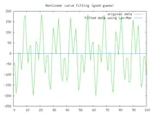
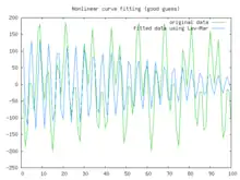
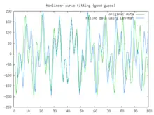
In this example we try to fit the function $y=a\cos \left(bX\right)+b\sin \left(aX\right)$ using the Levenberg–Marquardt algorithm implemented in GNU Octave as the leasqr function. The graphs show progressively better fitting for the parameters $a=100$ , $b=102$ used in the initial curve. Only when the parameters in the last graph are chosen closest to the original, are the curves fitting exactly. This equation is an example of very sensitive initial conditions for the Levenberg–Marquardt algorithm. One reason for this sensitivity is the existence of multiple minima — the function $\cos \left(\beta x\right)$ has minima at parameter value ${\hat {\beta }}$ and ${\hat {\beta }}+2n\pi$ .

References

Levenberg, Kenneth (1944). "A Method for the Solution of Certain Non-Linear Problems in Least Squares". Quarterly of Applied Mathematics. 2 (2): 164–168. doi:10.1090/qam/10666.
Marquardt, Donald (1963). "An Algorithm for Least-Squares Estimation of Nonlinear Parameters". SIAM Journal on Applied Mathematics. 11 (2): 431–441. doi:10.1137/0111030. hdl:10338.dmlcz/104299.
Girard, André (1958). "Excerpt from Revue d'optique théorique et instrumentale". Rev. Opt. 37: 225–241, 397–424.
Wynne, C. G. (1959). "Lens Designing by Electronic Digital Computer: I". Proc. Phys. Soc. Lond. 73 (5): 777–787. Bibcode:1959PPS....73..777W. doi:10.1088/0370-1328/73/5/310.
Morrison, David D. (1960). "Methods for nonlinear least squares problems and convergence proofs". Proceedings of the Jet Propulsion Laboratory Seminar on Tracking Programs and Orbit Determination: 1–9.
Wiliamowski, Bogdan; Yu, Hao (June 2010). "Improved Computation for Levenberg–Marquardt Training" (PDF). IEEE Transactions on Neural Networks and Learning Systems. 21 (6).
Transtrum, Mark K; Machta, Benjamin B; Sethna, James P (2011). "Geometry of nonlinear least squares with applications to sloppy models and optimization". Physical Review E. APS. 83 (3): 036701. arXiv:1010.1449. Bibcode:2011PhRvE..83c6701T. doi:10.1103/PhysRevE.83.036701. PMID 21517619. S2CID 15361707.
Transtrum, Mark K; Sethna, James P (2012). "Improvements to the Levenberg-Marquardt algorithm for nonlinear least-squares minimization". arXiv:1201.5885 [physics.data-an].
"Nonlinear Least-Squares Fitting". GNU Scientific Library. Archived from the original on 2020-04-14.
Kanzow, Christian; Yamashita, Nobuo; Fukushima, Masao (2004). "Levenberg–Marquardt methods with strong local convergence properties for solving nonlinear equations with convex constraints". Journal of Computational and Applied Mathematics. 172 (2): 375–397. Bibcode:2004JCoAM.172..375K. doi:10.1016/j.cam.2004.02.013.

External links

Detailed description of the algorithm can be found in Numerical Recipes in C, Chapter 15.5: Nonlinear models
C. T. Kelley, Iterative Methods for Optimization, SIAM Frontiers in Applied Mathematics, no 18, 1999, ISBN 0-89871-433-8. Online copy
History of the algorithm in SIAM news
A tutorial by Ananth Ranganathan
K. Madsen, H. B. Nielsen, O. Tingleff, Methods for Non-Linear Least Squares Problems (nonlinear least-squares tutorial; L-M code: analytic Jacobian secant)
T. Strutz: Data Fitting and Uncertainty (A practical introduction to weighted least squares and beyond). 2nd edition, Springer Vieweg, 2016, ISBN 978-3-658-11455-8.
H. P. Gavin, The Levenberg-Marquardt method for nonlinear least-squares curve-fitting problems (MATLAB implementation included)

This article is issued from Wikipedia. The text is licensed under Creative Commons - Attribution - Sharealike. Additional terms may apply for the media files.

[Levenberg-1] Levenberg, Kenneth (1944). "A Method for the Solution of Certain Non-Linear Problems in Least Squares". Quarterly of Applied Mathematics. 2 (2): 164–168. doi:10.1090/qam/10666.

[Marquardt-2] Marquardt, Donald (1963). "An Algorithm for Least-Squares Estimation of Nonlinear Parameters". SIAM Journal on Applied Mathematics. 11 (2): 431–441. doi:10.1137/0111030. hdl:10338.dmlcz/104299.

[Girard-3] Girard, André (1958). "Excerpt from Revue d'optique théorique et instrumentale". Rev. Opt. 37: 225–241, 397–424.

[Wynne-4] Wynne, C. G. (1959). "Lens Designing by Electronic Digital Computer: I". Proc. Phys. Soc. Lond. 73 (5): 777–787. Bibcode:1959PPS....73..777W. doi:10.1088/0370-1328/73/5/310.

[Morrison-5] Morrison, David D. (1960). "Methods for nonlinear least squares problems and convergence proofs". Proceedings of the Jet Propulsion Laboratory Seminar on Tracking Programs and Orbit Determination: 1–9.

[6] Wiliamowski, Bogdan; Yu, Hao (June 2010). "Improved Computation for Levenberg–Marquardt Training" (PDF). IEEE Transactions on Neural Networks and Learning Systems. 21 (6).

[Transtrum2011-7] Transtrum, Mark K; Machta, Benjamin B; Sethna, James P (2011). "Geometry of nonlinear least squares with applications to sloppy models and optimization". Physical Review E. APS. 83 (3): 036701. arXiv:1010.1449. Bibcode:2011PhRvE..83c6701T. doi:10.1103/PhysRevE.83.036701. PMID 21517619. S2CID 15361707.

[Transtrum2012-8] Transtrum, Mark K; Sethna, James P (2012). "Improvements to the Levenberg-Marquardt algorithm for nonlinear least-squares minimization". arXiv:1201.5885 [physics.data-an].

[9] "Nonlinear Least-Squares Fitting". GNU Scientific Library. Archived from the original on 2020-04-14.

[10] Kanzow, Christian; Yamashita, Nobuo; Fukushima, Masao (2004). "Levenberg–Marquardt methods with strong local convergence properties for solving nonlinear equations with convex constraints". Journal of Computational and Applied Mathematics. 172 (2): 375–397. Bibcode:2004JCoAM.172..375K. doi:10.1016/j.cam.2004.02.013.