Lindahl tax
A Lindahl tax is a form of taxation conceived by Erik Lindahl in which individuals pay for public goods according to their marginal benefits. In other words, they pay according to the amount of satisfaction or utility they derive from the consumption of an additional unit of the public good. Lindahl taxation is designed to maximize efficiency for each individual and provide the optimal level of a public good.
| Part of a series on |
| Taxation |
|---|
 |
| An aspect of fiscal policy |
Lindahl taxes can be seen as an individual's share of the collective tax burden of an economy. The optimal level of a public good is that quantity at which the willingness to pay for one more unit of the good, taken in totality for all the individuals is equal to the marginal cost of supplying that good. Lindahl tax is the optimal quantity times the willingness to pay for one more unit of that good at this quantity.[1]
History
The idea of using aggregate marginal utility in the analysis of public finance was not new in Europe. Knut Wicksell was one of the most prominent economists who studied this concept, eventually arguing that no individual should be forced to pay for any activity that does not give them utility.[2] Erik Lindahl was deeply influenced by Wicksell, who was his professor and mentor, and proposed a method for financing public goods in order to show that consensus politics is possible. As people are different in nature, their preferences are different, and consensus requires each individual to pay a somewhat different tax for every service, or good that he consumes. If each person's tax price is set equal to the marginal benefits received at the ideal service level, each person is made better off by provision of the public good and may accordingly agree to have that service level provided.
Lindahl equilibrium
A Lindahl equilibrium is a state of economic equilibrium under a Lindahl tax as well as a method for finding the optimum level for the supply of public goods or services that happens when the total per-unit price paid by each individual equals the total per-unit cost of the public good. It can be shown that an equilibrium exists for different environments.[3] Therefore, the Lindahl equilibrium describes how efficiency can be sustained in an economy with personalized prices. Leif Johansen gave the complete interpretation of the concept of "Lindahl equilibrium", which assumes that household consumption decisions are based on the share of the cost they must provide for the supply of the particular public good.[4]
This method of taxation for public goods is an equilibrium for two reasons. First, individuals are willing to pay the respective taxes for the quantity of public goods provided. Second, the cost of the public good is covered by the aggregate taxes. Therefore, the Lindahl pricing centers around the benefit principle, in which individuals are taxed based on their valuation of the benefit received from the good. This equilibrium is also the efficient level of public goods, as the social marginal benefit is equivalent to the social marginal cost.[5]
The importance of Lindahl equilibrium is that it fulfills the Samuelson condition and is therefore Pareto efficient,[3] despite the good in question being a public one. It also demonstrates how efficiency can be reached in an economy with public goods by the use of personalized prices. The personalized prices equate the individual valuation for a public good to the cost of the public good.
Lindahl equilibrium in an economy with only a public good
Lindahl and Samuelson defined the Lindahl equilibrium in a general economy, in which there are both public and private goods. Fain, Goel and Mungala[6] present a specialized definition, for the case in which there are only public goods.
- There is a fixed budget B, and k types of divisible public goods.
- The goal is to decide on an allocation x of the budget, such that x1+...+xk = B.
- There are n agents; each agent i has a utility function Ui over possible allocations of the budget.
An allocation x is a Lindahl equilibrium if there exist personal price-vectors p1,...,pn such that the following two conditions hold:
- For every agent i, the allocation x maximizes the utility Ui(x) subject to . That is: x is the best bundle that agent i could buy with his proportional share of the budget and his personal prices. In other words: if each agent chooses the best public bundle he can afford given his personal prices, then all agents unanimously choose the same public bundle.
- The allocation x maximizes the profit, defined as . Intuitively, it is assumed that some producer can produce public goods in cost 1, and he sells them to the public; his profit is the total amount of money he gains from selling the goods in the given prices, minus the total cost of production.
The personalized price-vector pi can be interpreted as the Lindahl tax on agent i.
Note the difference from a competitive equilibrium in a market of private goods (Fisher market):
- In a Fisher market equilibrium, there is a single price-vector for all agents, but each agent has a different bundle
- In a Lindahl equilibrium, there is a personal price-vector for each agent, but all agents have the same bundle.
A Lindahl equilibrium allocation in a market of public goods has a characterization without the price-vectors.[6]: Thm.2.1 Specifically, an allocation x is a Lindahl equilibrium if and only if, for every good j, , where the inequality becomes an equality when .
Existence
Foley[7] proved that, If the utility functions have continuous derivatives, are strictly increasing, and are strictly concave, then a Lindahl equilibrium exists in the general case of mixed public and private goods, and moreover, it lies in the fractional core. However, his proof is existential and does not provide an efficient algorithm.
Manipulation
The mechanism that, given agents' utilities, computes the Lindahl equilibrium, is not strategyproof, even in the setting with only public goods. This is a special case of the free-rider problem.
Computation
Fain, Goel and Mungala[6]: Thm.2.2 present an algorithm for computing the Lindahl equilibrium using convex programming, in the special case in which agents have scalar-separable non-satiating utilities. Particularly:
- If the agents' utilities are homogeneous of degree 1 and concave, the Lindahl equilibrium allocation can be computed by maxizing the Nash welfare .[6]: Cor.2.3 present Moreover, the gradient of this objective function can be computed using quadratic voting.
- For more general non-satiating utility functions, the Lindahl equilibrium can be computed by maximizing a potential function, that can be seen as a regularized version of the Nash welfare.
Discrete Lindahl equilibrium
Peters, PIerczynski, Shah and Skowron[8] present an adaptation of the concept of Lindahl equilibrium to a market with indivisible public goods. In this setting, a Lindahl equilibrium may be not Pareto-efficient.
- Example: there are three goods (a, b1, b2) and two voters, where Alice values a, b1 at 1 and b2 at 0, and George values a, b2 at 1 and b1 at 0. The budget of each agent is 3, and the cost of each good is 2. Producing only {a} is a Lindahl equilibrium, with prices for Alice: 2-0.009, 2-0.006, 0.001 and prices for George: 2-0.009, 0.001, 2-0.006. This is because (1) it maximizes the profit: the producer would not gain from producing b1 or b2; (2) it maximizes the agents' utilities: no agent can afford another desirable good. But {a} is not efficient, since it is dominated by {a,b1,b2}.
If the definition is strengthened to require that the total payment for each public good exactly equals its cost, then the stronger Lindahl equilibrium notion is equivalent to a concept they call strict stable priceability. A stable-priceable committee does not always exist, but extensive simulation experiments show that an "almost" stable-priceable committee almost always exists. It is possible to check in polynomial time whether a given committee is stable-priceable.
Lindahl Model

In the Lindahl Model, Dt represents the aggregate marginal benefit curve, which is the sum of Da and Db---the marginal benefits for the two individuals in the economy. In a Lindahl equilibrium, the optimal quantity of the public good will be where the social marginal benefit intersects the marginal cost (point P). Each individual's Lindahl tax rate will be based on their own marginal benefit curve. In this model, individual B will pay the price level at R and individual A will pay at point J.
Criticism
In theory, Lindahl pricing and taxation leads to an efficient provision of public goods. However, it requires the knowledge of the demand functions for each individual, and therefore is difficult to implement in practice. There are three main problems with the implementation of a Lindahl tax.
Preference revelation problem
When information about marginal benefits is available only from the individuals themselves, they tend to under report their valuation for a particular good. In doing this, an individual can lower his or her tax cost by under reporting the benefits derived from the public good or service. The incentive to lie is associated with the free rider problem; if an individual reports a lower benefit, he or she will pay less taxes, but only see a marginal decrease in the public good. This informational problem shows that survey-based Lindahl taxation is not incentive compatible. Incentives to understate or under report one's true benefits under Lindahl taxation resemble those of a traditional public goods game.[5]
Preference revelation mechanisms can be used to solve that problem,[9][10] although none of these has been shown to completely and satisfactorily address it. The Vickrey–Clarke–Groves mechanism is an example of this, ensuring true values are revealed and that a public good is provided only when it should be. The allocation of cost is taken as given and the consumers will report their net benefits (benefits-cost) the public good will be provided if the sum of the net benefits of all consumers is positive. If the public good is provided side payments will be made reflecting the fact that truth telling is costly. The side payments internalize the net benefit of the public good to other players. The side payments must be financed from outside the mechanism. In reality, preference revelation is difficult as the size of the population makes it costly both in terms of money and time.[11]
Preference knowledge problem
A second drawback to the Lindahl solution is that individuals may be unsure of their own valuation of a public good. Even if individuals are attempting to be honest with their willingness to pay, they may have no idea of their true value. This is especially true for public goods that individuals do not interact with on a day-to-day basis, like fireworks and national defense.[11]
Preference aggregation problem
Even if individuals know their marginal willingness to pay, and are honest in their reporting, the government can have extreme difficulties aggregating this into a social value. In situations where few individuals are affected by the public good, like the example below, aggregation can be relatively simple. However, in the case of national defense in the United States, compiling the marginal willingness to pay for this public good of each individual would be nearly impossible.[11]
Mathematical representation
We assume that there are two goods in an economy:the first one is a "public good", and the second is "everything else". The price of the public good can be assumed to be Ppublic and the price of everything else can be Pelse. Person 1 will choose his bundle such that:
- α*P(public)/P(else) = MRS(person1)
This is just the usual price ratio/marginal rate of substitution deal; the only change is that we multiply Ppublic by α to allow for the price adjustment to the public good. Similarly, Person 2 will choose his bundle such that:
- (1-ɑ)*P(public)/P(else)= MRS(person2)
Now we have both individuals' utility maximizing. We know that in a competitive equilibrium, the marginal cost ratio or price ratio should be equal to the marginal rate of transformation, or
- MC(public)/MC(else)=[P(public)/P(else)]=MRT
Example
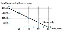
Take for example a public park, with a constant marginal cost of $15 per acre. This public park will be available to two people, Sarah and Tom.

Figure 1 shows Sarah's marginal willingness to pay for a public park. For the first acre of the park, Sarah is willing to pay $20. For the 80th acre, her marginal willingness to pay has decreased down to zero.

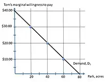
Figure 2 shows Tom's marginal willingness to pay for a public park. Unlike Sarah, for the first acre of park he is willing to pay $40, and for the 40th acre of park he has a marginal willingness to pay of $20. For the 80th acre of park his marginal willingness to pay is zero.

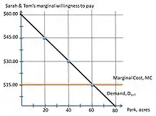
Figure 3 shows the aggregate marginal willingness to pay for the public park. As seen on the figure, Sarah and Tom together are willing to pay $60 for the first acre of park. This is higher than the marginal cost of the first acre ($15) and therefore this first acre of park should be produced. Sarah and Tom together are willing to pay $45 for the 20th acre, and $30 for the 40th acre, which are both again above the marginal cost of $15. The marginal cost curve intersects their aggregate willingness to pay curve at the 60th acre, when they are together willing to pay the $15 marginal cost. Thus, the Lindahl equilibrium involves charging Sarah $5 and Tom $10 for each of the 60 acres of park.[5]
Sources
Citations
- Equity: In Theory and Practice, p. 103.
- Roberts, Donald John (1974-02-01). "The Lindahl solution for economies with public goods". Journal of Public Economics. 3 (1): 23–42. doi:10.1016/0047-2727(74)90021-8. ISSN 0047-2727.
- Mark Walker, "Lindahl Equilibrium", University of Arizona
- Leif Johansen (September 1963). "Some Notes on the Lindahl Theory of Determination of Public Expenditures". International Economic Review. 4 (3): 346–58. doi:10.2307/2525312. JSTOR 2525312.
- Gruber, Jonathan (2016). Public Finance and Public Policy (Fifth ed.). Worth Publishers, Incorporated. pp. 243–246. ISBN 9781464143335.
- Fain, Brandon; Goel, Ashish; Munagala, Kamesh (2016). Cai, Yang; Vetta, Adrian (eds.). "The Core of the Participatory Budgeting Problem". Web and Internet Economics. Lecture Notes in Computer Science. Springer Berlin Heidelberg. 10123: 384–399. arXiv:1610.03474. doi:10.1007/978-3-662-54110-4_27. ISBN 9783662541104. S2CID 13443635.. Note that what they call "core" is often called the "weak core".
- Foley, Duncan K. (1970). "Lindahl's Solution and the Core of an Economy with Public Goods". Econometrica. 38 (1): 66–72. doi:10.2307/1909241. ISSN 0012-9682.
- Peters, Dominik; Pierczynski, Grzegorz; Shah, Nisarg; Skowron, Piotr (2021). "Market-Based Explanations of Collective Decisions". Proceedings of the 35th AAAI Conference on Artificial Intelligence. AAAI'21. 35 (6): 5656–5663. doi:10.1609/aaai.v35i6.16710. S2CID 222132258.
- Revelation, Demand. "Demand Revelation". Economic Theory. Retrieved 30 September 2011.
- "Fred Foldvary on Demand Revelation: Better than Voting" Archived 2012-04-02 at the Wayback Machine
- Backhaus, Jürgen Georg, Wagner, Richard E. (2004). Handbook of Public Finance. ISBN 978-1-4020-7863-7.
{{cite book}}: CS1 maint: multiple names: authors list (link)
References and further reading
- Foley, Duncan K. (1970), "Lindahl's Solution and the Core of an Economy with Public Goods" (PDF), Econometrica, 38 (1): 66–72, doi:10.2307/1909241, hdl:1721.1/63828, JSTOR 1909241.
- "Public Economics" by Gareth D. Myles (October 2001)
- Laffont, Jean-Jacques (1988). "2.4 Lindahl equilibrium, 2.5.3 Majority voting or the law of the median voter". Fundamentals of public economics. MIT. pp. 41–43, 51–53. ISBN 978-0-262-12127-9.
{{cite book}}: External link in|publisher= - Lindahl, Erik (1958) [1919], "Just taxation – A positive solution", in Musgrave, R. A.; Peacock, A. T. (eds.), Classics in the Theory of Public Finance, London: Macmillan.
- Salanié, Bernard (2000). "5.2.3 The Lindahl equilibrium". Microeconomics of market failures (English translation of the (1998) French Microéconomie: Les défaillances du marché (Economica, Paris) ed.). Cambridge, MA: MIT Press. pp. 74–75. ISBN 978-0-262-19443-3.
- Starrett, David A. (1988). "5 Planning mechanisms, 16 Practical methods for large project evaluation (Groves–Clarke mechanism)". Foundations of public economics. Cambridge economic handbooks. Vol. XVI. Cambridge: Cambridge University Press. pp. 65–72, 270–71. ISBN 9780521348010.