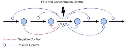
Metabolic control analysis

A control coefficient[7] [8][9] measures the relative steady state change in a system variable, e.g. pathway flux (J) or metabolite concentration (S), in response to a relative change in a parameter, e.g. enzyme activity or the steady-state rate (${\displaystyle v_{i}}$) of step ${\displaystyle i}$. The two main control coefficients are the flux and concentration control coefficients. Flux control coefficients are defined by

${\displaystyle C_{v_{i}}^{J}=\left({\frac {dJ}{dp}}{\frac {p}{J}}\right){\bigg /}\left({\frac {\partial v_{i}}{\partial p}}{\frac {p}{v_{i}}}\right)={\frac {d\ln J}{d\ln v_{i}}}}$

and concentration control coefficients by

${\displaystyle C_{v_{i}}^{S}=\left({\frac {dS}{dp}}{\frac {p}{S}}\right){\bigg /}\left({\frac {\partial v_{i}}{\partial p}}{\frac {p}{v_{i}}}\right)={\frac {d\ln S}{d\ln v_{i}}}}$

Control coefficients measure the effect of perturbations in an enzyme on a steady-state observable such as a flux or metabolite concentration. Note that the effect of a perturbation can be positive or negative depending on context. In the figure, a perturbation is assumed to be at step three. Figure modified and redrawn from[10]

.

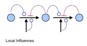
The elasticity coefficient measures the local response of an enzyme or other chemical reaction to changes in its environment. Such changes include factors such as substrates, products, or effector concentrations. For further information, please refer to the dedicated page at elasticity coefficients.

Elasticities are local quantities that measure the effect of substrates, products, and effectors on a given reaction. The vertical black arrows represent enzyme catalysis. Figure redrawn and modified from[11]

.

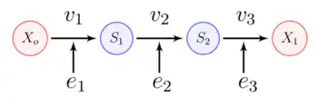
It is possible to combine the summation with the connectivity theorems to obtain closed expressions that relate the control coefficients to the elasticity coefficients. For example, consider the simplest non-trivial pathway:

${\displaystyle X_{o}\rightarrow S\rightarrow X_{1}}$

We assume that ${\displaystyle X_{o}}$ and ${\displaystyle X_{1}}$ are fixed boundary species so that the pathway can reach a steady state. Let the first step have a rate ${\displaystyle v_{1}}$ and the second step ${\displaystyle v_{2}}$. Focusing on the flux control coefficients, we can write one summation and one connectivity theorem for this simple pathway:

${\displaystyle C_{v_{1}}^{J}+C_{v_{2}}^{J}=1}$

${\displaystyle C_{v_{1}}^{J}\varepsilon _{S}^{v_{1}}+C_{v_{2}}^{J}\varepsilon _{S}^{v_{2}}=0}$

Using these two equations we can solve for the flux control coefficients to yield

${\displaystyle C_{v_{1}}^{J}={\frac {\varepsilon _{S}^{2}}{\varepsilon _{S}^{2}-\varepsilon _{S}^{1}}}}$

${\displaystyle C_{v_{2}}^{J}={\frac {-\varepsilon _{S}^{1}}{\varepsilon _{S}^{2}-\varepsilon _{S}^{1}}}}$

Using these equations we can look at some simple extreme behaviors. For example, let us assume that the first step is completely insensitive to its product (i.e. not reacting with it), S, then ${\displaystyle \varepsilon _{S}^{v_{1}}=0}$. In this case, the control coefficients reduce to

${\displaystyle C_{v_{1}}^{J}=1}$

${\displaystyle C_{v_{2}}^{J}=0}$

That is all the control (or sensitivity) is on the first step. This situation represents the classic rate-limiting step that is frequently mentioned in text books. The flux through the pathway is completely dependent on the first step. Under these conditions, no other step in the pathway can affect the flux. The effect is however dependent on the complete insensitivity of the first step to its product. Such a situation is likely to be rare in real pathways. In fact the classic rate limiting step has almost never been observed experimentally. Instead, a range of limitingness is observed, with some steps having more limitingness (control) than others.

We can also derive the concentration control coefficients for the simple two step pathway:

${\displaystyle C_{v_{1}}^{S}={\frac {1}{\varepsilon _{S}^{2}-\varepsilon _{S}^{1}}}}$

${\displaystyle C_{v_{2}}^{S}={\frac {-1}{\varepsilon _{S}^{2}-\varepsilon _{S}^{1}}}}$

Consider the simple three step pathway:

${\displaystyle X_{o}\rightarrow S_{1}\rightarrow S_{2}\rightarrow X_{1}}$

where ${\displaystyle X_{o}}$ and ${\displaystyle X_{1}}$ are fixed boundary species, the control equations for this pathway can be derived in a similar manner to the simple two step pathway although it is somewhat more tedious.

${\displaystyle C_{e_{1}}^{J}=\varepsilon _{1}^{2}\varepsilon _{2}^{3}/D}$

${\displaystyle C_{e_{2}}^{J}=-\varepsilon _{1}^{1}\varepsilon _{2}^{3}/D}$

${\displaystyle C_{e_{3}}^{J}=\varepsilon _{1}^{1}\varepsilon _{2}^{2}/D}$

where D the denominator is given by

${\displaystyle D=\varepsilon _{1}^{2}\varepsilon _{2}^{3}-\varepsilon _{1}^{1}\varepsilon _{2}^{3}+\varepsilon _{1}^{1}\varepsilon _{2}^{2}}$

Note that every term in the numerator appears in the denominator, this ensures that the flux control coefficient summation theorem is satisfied.

Likewise the concentration control coefficients can also be derived, for ${\displaystyle S_{1}}$

${\displaystyle C_{e_{1}}^{S_{1}}=(\varepsilon _{2}^{3}-\varepsilon _{2}^{2})/D}$

${\displaystyle C_{e_{2}}^{S_{1}}=-\varepsilon _{2}^{3}/D}$

${\displaystyle C_{e_{3}}^{S_{1}}=\varepsilon _{2}^{2}/D}$

And for ${\displaystyle S_{2}}$

${\displaystyle C_{e_{1}}^{S_{2}}=\varepsilon _{1}^{2}/D}$

${\displaystyle C_{e_{2}}^{S_{2}}=-\varepsilon _{1}^{1}/D}$

${\displaystyle C_{e_{3}}^{S_{2}}=(\varepsilon _{1}^{1}-\varepsilon _{1}^{2})/D}$

Note that the denominators remain the same as before and behave as a normalizing factor.

Control equations can also be derived by considering the effect of perturbations on the system. Consider that reaction rates ${\displaystyle v_{1}}$ and ${\displaystyle v_{2}}$ are determined by two enzymes ${\displaystyle e_{1}}$ and ${\displaystyle e_{2}}$ respectively. Changing either enzyme will result in a change to the steady state level of ${\displaystyle x}$ and the steady state reaction rates ${\displaystyle v}$. Consider a small change in ${\displaystyle e_{1}}$ of magnitude ${\displaystyle \delta e_{1}}$. This will have a number of effects, it will increase ${\displaystyle v_{1}}$ which in turn will increase ${\displaystyle x}$ which in turn will increase ${\displaystyle v_{2}}$. Eventually the system will settle to a new steady state. We can describe these changes by focusing on the change in ${\displaystyle v_{1}}$ and ${\displaystyle v_{2}}$. The change in ${\displaystyle v_{2}}$, which we designate ${\displaystyle \delta v_{2}}$, came about as a result of the change ${\displaystyle \delta x}$. Because we are only considering small changes we can express the change ${\displaystyle \delta v_{2}}$ in terms of ${\displaystyle \delta x}$ using the relation

${\displaystyle \delta v_{2}={\frac {\partial v_{2}}{\partial x}}\delta x}$

where the derivative ${\displaystyle \partial v_{2}/\partial x}$ measures how responsive ${\displaystyle v_{2}}$ is to changes in ${\displaystyle x}$. The derivative can be computed if we know the rate law for ${\displaystyle v_{2}}$. For example, if we assume that the rate law is ${\displaystyle v_{2}=k_{2}x}$ then the derivative is ${\displaystyle k_{2}}$. We can also use a similar strategy to compute the change in ${\displaystyle v_{1}}$ as a result of the change ${\displaystyle \delta e_{1}}$. This time the change in ${\displaystyle v_{1}}$ is a result of two changes, the change in ${\displaystyle e_{1}}$ itself and the change in ${\displaystyle x}$. We can express these changes by summing the two individual contributions:

${\displaystyle \delta v_{1}={\frac {\partial v_{1}}{\partial e_{1}}}\delta e_{1}+{\frac {\partial v_{1}}{\partial x}}\delta x}$

We have two equations, one describing the change in ${\displaystyle v_{1}}$ and the other in ${\displaystyle v_{2}}$. Because we allowed the system to settle to a new steady state we can also state that the change in reaction rates must be the same (otherwise it wouldn't be at steady state). That is we can assert that ${\displaystyle \delta v_{1}=\delta v_{2}}$. With this in mind we equate the two equations and write

${\displaystyle {\frac {\partial v_{2}}{\partial x}}\delta x={\frac {\partial v_{1}}{\partial e_{1}}}\delta e_{1}+{\frac {\partial v_{1}}{\partial x}}\delta x}$

Solving for the ratio ${\displaystyle \delta x/\delta e_{1}}$ we obtain:

${\displaystyle {\frac {\delta x}{\delta e_{1}}}={\dfrac {-{\dfrac {\partial v_{1}}{\partial e_{1}}}}{{\dfrac {\partial v_{2}}{\partial x}}-{\dfrac {\partial v_{1}}{\partial x}}}}}$

In the limit, as we make the change ${\displaystyle \delta e_{1}}$ smaller and smaller, the left-hand side converges to the derivative ${\displaystyle dx/de_{1}}$:

${\displaystyle \lim _{\delta e_{1}\rightarrow 0}{\frac {\delta x}{\delta e_{1}}}={\frac {dx}{de_{1}}}={\dfrac {-{\dfrac {\partial v_{1}}{\partial e_{1}}}}{{\dfrac {\partial v_{2}}{\partial x}}-{\dfrac {\partial v_{1}}{\partial x}}}}}$

We can go one step further and scale the derivatives to eliminate units. Multiplying both sides by ${\displaystyle e_{1}}$ and dividing both sides by ${\displaystyle x}$ yields the scaled derivatives:

${\displaystyle {\frac {dx}{de_{1}}}{\frac {e_{1}}{x}}={\frac {-{\dfrac {\partial v_{1}}{\partial e_{1}}}{\dfrac {e_{1}}{v_{1}}}}{{\dfrac {\partial v_{2}}{\partial x}}{\dfrac {x}{v_{2}}}-{\dfrac {\partial v_{1}}{\partial x}}{\dfrac {x}{v_{1}}}}}}$

The scaled derivatives on the right-hand side are the elasticities, ${\displaystyle \varepsilon _{x}^{v}}$ and the scaled left-hand term is the scaled sensitivity coefficient or concentration control coefficient, ${\displaystyle C_{e}^{x}}$

${\displaystyle C_{e_{1}}^{x}={\frac {\varepsilon _{e_{1}}^{1}}{\varepsilon _{x}^{2}-\varepsilon _{x}^{1}}}}$

We can simplify this expression further. The reaction rate ${\displaystyle v_{1}}$ is usually a linear function of ${\displaystyle e_{1}}$. For example, in the Briggs–Haldane equation, the reaction rate is given by ${\displaystyle v=e_{1}k_{cat}x/(K_{m}+x)}$. Differentiating this rate law with respect to ${\displaystyle e_{1}}$ and scaling yields ${\displaystyle \varepsilon _{e_{1}}^{v_{1}}=1}$.

Using this result gives:

${\displaystyle C_{e_{1}}^{x}={\frac {1}{\varepsilon _{x}^{2}-\varepsilon _{x}^{1}}}}$

A similar analysis can be done where ${\displaystyle e_{2}}$ is perturbed. In this case we obtain the sensitivity of ${\displaystyle x}$ with respect to ${\displaystyle e_{2}}$:

${\displaystyle C_{e_{2}}^{x}=-{\frac {1}{\varepsilon _{x}^{2}-\varepsilon _{x}^{1}}}}$

The above expressions measure how much enzymes ${\displaystyle e_{1}}$ and ${\displaystyle e_{2}}$ control the steady state concentration of intermediate ${\displaystyle x}$. We can also consider how the steady state reaction rates ${\displaystyle v_{1}}$ and ${\displaystyle v_{2}}$ are affected by perturbations in ${\displaystyle e_{1}}$ and ${\displaystyle e_{2}}$. This is often of importance to metabolic engineers who are interested in increasing rates of production. At steady state the reaction rates are often called the fluxes and abbreviated to ${\displaystyle J_{1}}$ and ${\displaystyle J_{2}}$. For a linear pathway such as this example, both fluxes are equal at steady-state so that the flux through the pathway is simply referred to as ${\displaystyle J}$. Expressing the change in flux as a result of a perturbation in ${\displaystyle e_{1}}$ and taking the limit as before we obtain

${\displaystyle C_{e_{1}}^{J}={\frac {\varepsilon _{x}^{1}}{\varepsilon _{x}^{2}-\varepsilon _{x}^{1}}},\quad C_{e_{2}}^{J}={\frac {-\varepsilon _{x}^{1}}{\varepsilon _{x}^{2}-\varepsilon _{x}^{1}}}}$

The above expressions tell us how much enzymes ${\displaystyle e_{1}}$ and ${\displaystyle e_{2}}$ control the steady state flux. The key point here is that changes in enzyme concentration, or equivalently the enzyme activity, must be brought about by an external action.

A linear chain of enzyme-catalyzed reaction steps without a negative feedback loop is the simplest pathway to consider. The figure below shows a three-step linear chain.

Linear chain of four reactions catalyzed by enzymes e1 to e4

We can assume that each reaction is reversible and that the boundary species, ${\displaystyle X_{o}}$ and ${\displaystyle X_{1}}$ are fixed so that the pathway can reach a steady-state.

Analytical solutions for the control coefficients can be obtained if we assume simple mass-action kinetics on each reaction step:

${\displaystyle v_{i}=k_{i}s_{i-1}-k_{-i}s_{i}}$

where ${\displaystyle k_{i}}$ and ${\displaystyle k_{-1}}$ are the forward and reverse rate-constants respectively. ${\displaystyle s_{i-1}}$ is the substrate and ${\displaystyle s_{i}}$ the product. If we recall that the equilibrium constant for this simple reaction is:

${\displaystyle K_{eq}=q_{i}={\frac {k_{i}}{k_{-i}}}={\frac {s_{i}}{s_{i-1}}}}$

we can modify the mass-action kinetic equation to be:

${\displaystyle v_{i}=k_{i}\left(s_{i-1}-{\frac {s_{i}}{q_{i}}}\right)}$

Given the reaction rates, the differential equations describing the rates of change of the species can be described. For example, the rate of change of ${\displaystyle s_{1}}$ will equal:

${\displaystyle {\frac {ds_{1}}{dt}}=k_{1}\left(x_{0}-{\frac {s_{1}}{q_{1}}}\right)-k_{2}\left(s_{1}-{\frac {s_{2}}{q_{2}}}\right)}$

By setting the differential equations to zero, the steady-state concentration for the species can be derived, from which the pathway flux equation can also be determined. For the three-step pathway, the steady-state concentrations of ${\displaystyle s_{1}}$ and ${\displaystyle s_{2}}$ are given by:

${\displaystyle {\begin{aligned}&s_{1}={\frac {q_{1}}{q_{3}}}{\frac {k_{2}k_{3}x_{1}+k_{1}k_{2}q_{3}x_{o}+k_{1}k_{3}q_{2}q_{3}x_{o}}{k_{1}k_{2}+k_{1}k_{3}q_{2}+k_{2}k_{3}q_{1}q_{2}}}\\[6pt]&s_{2}={\frac {q_{2}}{q_{3}}}{\frac {k_{1}k_{3}x_{1}+k_{2}k_{3}q_{1}x_{1}+k_{1}k_{2}q_{1}q_{3}x_{o}}{k_{1}k_{2}+k_{1}k_{3}q_{2}+k_{2}k_{3}q_{1}q_{2}}}\end{aligned}}}$

Inserting either ${\displaystyle s_{1}}$ or ${\displaystyle s_{2}}$ into one of the rate laws will give the steady-state pathway flux, ${\displaystyle J}$:

${\displaystyle J={\frac {x_{o}q_{1}q_{2}q_{3}-x_{1}}{{\frac {1}{k_{1}}}q_{1}q_{2}q_{3}+{\frac {1}{k_{2}}}q_{2}q_{3}+{\frac {1}{k_{3}}}q_{3}}}}$

A pattern can be seen in this equation such that, in general, for a linear pathway of ${\displaystyle n}$ steps, the steady-state pathway flux is given by:

${\displaystyle J={\frac {x_{o}\prod _{i=1}^{n}q_{i}-x_{1}}{\sum _{i=1}^{n}{\frac {1}{k_{i}}}\left(\prod _{j=i}^{n}q_{j}\right)}}}$

Note that the pathway flux is a function of all the kinetic and thermodynamic parameters. This means there is no single parameter that determines the flux completely. If ${\displaystyle k_{i}}$ is equated to enzyme activity, then every enzyme in the pathway has some influence over the flux. Given the flux expression, it is possible to derive the flux control coefficients by differentiation and scaling of the flux expression. This can be done for the general case of ${\displaystyle n}$ steps:

${\displaystyle C_{i}^{J}={\frac {{\frac {1}{k_{i}}}\prod _{j=i}^{n}q_{j}}{\sum _{j=1}^{n}{\frac {1}{k_{j}}}\prod _{k=j}^{n}q_{k}}}}$

This result yields two corollaries:

• The sum of the flux control coefficients is one. This confirms the summation theorem.
• The value of an individual flux control coefficient in a linear reaction chain is greater than 0 or less than one: ${\displaystyle 0\leq C_{i}^{J}\leq 1}$

For the three-step linear chain, the flux control coefficients are given by:

${\displaystyle C_{1}^{J}={\frac {1}{k_{1}}}{\frac {q_{1}q_{2}q_{3}}{d}};\quad C_{2}^{J}={\frac {1}{k_{2}}}{\frac {q_{2}q_{3}}{d}};\quad C_{3}^{J}={\frac {1}{k_{3}}}{\frac {q_{3}}{d}}}$

where ${\displaystyle d}$ is given by:

${\displaystyle d={\frac {1}{k_{1}}}q_{1}q_{2}q_{3}+{\frac {1}{k_{2}}}q_{2}q_{3}+{\frac {1}{k_{3}}}q_{3}}$

Given these results, there are some immediate observations:

• If all three steps have large equilibrium constants, that is ${\displaystyle q_{i}\gg 1}$, then ${\displaystyle C_{1}^{J}}$ tends to one and the remaining coefficients tend to zero.
• If the equilibrium constants are smaller, control tends to get distributed across all three steps.

The reason why control gets more distributed is that with more moderate equilibrium constants, perturbations can more easily travel upstream as well as downstream. For example, a perturbation at the last step, ${\displaystyle k_{3}}$, is better able to influence the reaction rates upstream, which results in an alteration in the steady-state flux.

An important result can be obtained if we set all ${\displaystyle k_{i}}$ equal to each other. Under these conditions, the flux control coefficient is proportional to the numerator. That is:

${\displaystyle {\begin{aligned}C_{1}^{J}&\propto q_{1}q_{2}q_{3}\\C_{2}^{J}&\propto q_{2}q_{3}\\C_{3}^{J}&\propto q_{3}\\\end{aligned}}}$

If we assume that the equilibrium constants are all greater than 1.0, then since earlier steps have more ${\displaystyle q_{i}}$ terms, it must mean that earlier steps will, in general, have high larger flux control coefficients. In a linear chain of reaction steps, flux control will tend to be biased towards the front of the pathway. From a metabolic engineering or drug-targeting perspective, preference should be given to targeting the earlier steps in a pathway since they have the greatest effect on pathway flux. Note that this rule only applies to pathways without negative feedback loops.[12]

There are a number of software tools that can directly compute elasticities and control coefficients:

• COPASI (GUI)
• PySCeS[13] (Python)
• SBW[14] (GUI)
• libroadrunner[15] (Python)
• VCell

Classical Control theory is a field of mathematics that deals with the control of dynamical systems in engineered processes and machines. In 2004 Brian Ingalls published a paper[16] that showed that classical control theory and metabolic control analysis were identical. The only difference was that metabolic control analysis was confined to zero frequency responses when cast in the frequency domain whereas classical control theory imposes no such restriction. The other significant difference is that classical control theory[17] has no notion of stoichiometry and conservation of mass which makes it more cumbersome to use but also means it fails to recognize the structural properties inherent in stoichiometric networks which provide useful biological insights.

• Branched pathways
• Biochemical systems theory
• Control coefficient (biochemistry)
• Flux (metabolism)
• Moiety conservation
• Rate-limiting step (biochemistry)

• The Metabolic Control Analysis Web

References

- Fell D., (1997) Understanding the Control of Metabolism, Portland Press.
- Heinrich R. and Schuster S. (1996) The Regulation of Cellular Systems, Chapman and Hall.
- Salter, M.; Knowles, R. G.; Pogson, C. I. (1994). "Metabolic control". Essays in Biochemistry. 28: 1–12. PMID 7925313.
- Ingalls, B. P. (2004) A Frequency Domain Approach to Sensitivity Analysis of Biochemical Systems, Journal of Physical Chemistry B, 108, 1143-1152.
- Savageau M.A (1976) Biochemical systems analysis: a study of function and design in molecular biology, Reading, MA, Addison–Wesley.
- Higgins, J. (1963). "Analysis of sequential reactions". Annals of the New York Academy of Sciences. 108 (1): 305–321. Bibcode:1963NYASA.108..305H. doi:10.1111/j.1749-6632.1963.tb13382.x. PMID 13954410. S2CID 30821044.
- Kacser, H.; Burns, J. A. (1973). "The control of flux". Symposia of the Society for Experimental Biology. 27: 65–104. PMID 4148886.
- Heinrich, R.; Rapoport, T. A. (1974). "A linear steady-state treatment of enzymatic chains. General properties, control and effector strength". European Journal of Biochemistry. 42 (1): 89–95. doi:10.1111/j.1432-1033.1974.tb03318.x. PMID 4830198.
- Burns, J.A.; Cornish-Bowden, A.; Groen, A.K.; Heinrich, R.; Kacser, H.; Porteous, J.W.; Rapoport, S.M.; Rapoport, T.A.; Stucki, J.W.; Tager, J.M.; Wanders, R.J.A.; Westerhoff, H.V. (1985). "Control analysis of metabolic systems". Trends Biochem. Sci. 10: 16. doi:10.1016/0968-0004(85)90008-8.
- Liebermeister, Wolfram (11 May 2022). "Structural Thermokinetic Modelling". Metabolites. 12 (5): 434. doi:10.3390/metabo12050434. PMC 9144996. PMID 35629936.
- Liebermeister, Wolfram (2016). "Optimal enzyme rhythms in cells". arXiv:1602.05167.
{{cite journal}}: Cite journal requires|journal=(help) - Heinrich R. and Schuster S. (1996) The Regulation of Cellular Systems, Chapman and Hall.
- Olivier, B. G.; Rohwer, J. M.; Hofmeyr, J.-H. S. (15 February 2005). "Modelling cellular systems with PySCeS". Bioinformatics. 21 (4): 560–561. doi:10.1093/bioinformatics/bti046. PMID 15454409.
- Bergmann, Frank T.; Sauro, Herbert M. (December 2006). "SBW - A Modular Framework for Systems Biology". Proceedings of the 2006 Winter Simulation Conference. pp. 1637–1645. doi:10.1109/WSC.2006.322938. ISBN 1-4244-0501-7.
- Choi, Kiri; Medley, J. Kyle; König, Matthias; Stocking, Kaylene; Smith, Lucian; Gu, Stanley; Sauro, Herbert M. (September 2018). "Tellurium: An extensible python-based modeling environment for systems and synthetic biology". Biosystems. 171: 74–79. doi:10.1016/j.biosystems.2018.07.006. PMC 6108935. PMID 30053414.
- Drengstig, Tormod; Kjosmoen, Thomas; Ruoff, Peter (19 May 2011). "On the Relationship between Sensitivity Coefficients and Transfer Functions of Reaction Kinetic Networks". The Journal of Physical Chemistry B. 115 (19): 6272–6278. doi:10.1021/jp200578e. PMID 21520979.
- Nise, Norman S. (2019). Control systems engineering (Eighth, Wiley abridged print companion ed.). Hoboken, NJ. ISBN 978-1119592921.
{{cite book}}: CS1 maint: location missing publisher (link)