Regularization (mathematics)
In mathematics, statistics, finance,[1] computer science, particularly in machine learning and inverse problems, regularization is a process that changes the result answer to be "simpler". It is often used to obtain results for ill-posed problems or to prevent overfitting.[2]
| Part of a series on |
| Machine learning and data mining |
|---|
 |

Although regularization procedures can be divided in many ways, the following delineation is particularly helpful:
- Explicit regularization is regularization whenever one explicitly adds a term to the optimization problem. These terms could be priors, penalties, or constraints. Explicit regularization is commonly employed with ill-posed optimization problems. The regularization term, or penalty, imposes a cost on the optimization function to make the optimal solution unique.
- Implicit regularization is all other forms of regularization. This includes, for example, early stopping, using a robust loss function, and discarding outliers. Implicit regularization is essentially ubiquitous in modern machine learning approaches, including stochastic gradient descent for training deep neural networks, and ensemble methods (such as random forests and gradient boosted trees).
In explicit regularization, independent of the problem or model, there is always a data term, that corresponds to a likelihood of the measurement and a regularization term that corresponds to a prior. By combining both using Bayesian statistics, one can compute a posterior, that includes both information sources and therefore stabilizes the estimation process. By trading off both objectives, one chooses to be more addictive to the data or to enforce generalization (to prevent overfitting). There is a whole research branch dealing with all possible regularizations. In practice, one usually tries a specific regularization and then figures out the probability density that corresponds to that regularization to justify the choice. It can also be physically motivated by common sense or intuition.
In machine learning, the data term corresponds to the training data and the regularization is either the choice of the model or modifications to the algorithm. It is always intended to reduce the generalization error, i.e. the error score with the trained model on the evaluation set and not the training data.[3]
One of the earliest uses of regularization is Tikhonov regularization, related to the method of least squares.
Classification
Empirical learning of classifiers (from a finite data set) is always an underdetermined problem, because it attempts to infer a function of any given only examples .
A regularization term (or regularizer) is added to a loss function:
where is an underlying loss function that describes the cost of predicting when the label is , such as the square loss or hinge loss; and is a parameter which controls the importance of the regularization term. is typically chosen to impose a penalty on the complexity of . Concrete notions of complexity used include restrictions for smoothness and bounds on the vector space norm.[4]
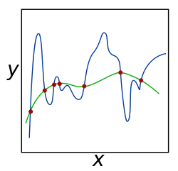
A theoretical justification for regularization is that it attempts to impose Occam's razor on the solution (as depicted in the figure above, where the green function, the simpler one, may be preferred). From a Bayesian point of view, many regularization techniques correspond to imposing certain prior distributions on model parameters.[5]
Regularization can serve multiple purposes, including learning simpler models, inducing models to be sparse and introducing group structure into the learning problem.
The same idea arose in many fields of science. A simple form of regularization applied to integral equations (Tikhonov regularization) is essentially a trade-off between fitting the data and reducing a norm of the solution. More recently, non-linear regularization methods, including total variation regularization, have become popular.
Generalization
Regularization can be motivated as a technique to improve the generalizability of a learned model.
The goal of this learning problem is to find a function that fits or predicts the outcome (label) that minimizes the expected error over all possible inputs and labels. The expected error of a function is:
where and are the domains of input data and their labels respectively.
Typically in learning problems, only a subset of input data and labels are available, measured with some noise. Therefore, the expected error is unmeasurable, and the best surrogate available is the empirical error over the available samples:
Without bounds on the complexity of the function space (formally, the reproducing kernel Hilbert space) available, a model will be learned that incurs zero loss on the surrogate empirical error. If measurements (e.g. of ) were made with noise, this model may suffer from overfitting and display poor expected error. Regularization introduces a penalty for exploring certain regions of the function space used to build the model, which can improve generalization.
Tikhonov regularization
These techniques are named for Andrey Nikolayevich Tikhonov, who applied regularization to integral equations and made important contributions in many other areas.
When learning a linear function , characterized by an unknown vector such that , one can add the -norm of the vector to the loss expression in order to prefer solutions with smaller norms. Tikhonov regularization is one of the most common forms. It is also known as ridge regression. It is expressed as:
- ,
where would represent samples used for training.
In the case of a general function, the norm of the function in its reproducing kernel Hilbert space is:
As the norm is differentiable, learning can be advanced by gradient descent.
Tikhonov-regularized least squares
The learning problem with the least squares loss function and Tikhonov regularization can be solved analytically. Written in matrix form, the optimal is the one for which the gradient of the loss function with respect to is 0.
By construction of the optimization problem, other values of give larger values for the loss function. This can be verified by examining the second derivative .
During training, this algorithm takes time. The terms correspond to the matrix inversion and calculating , respectively. Testing takes time.
Early stopping
Early stopping can be viewed as regularization in time. Intuitively, a training procedure such as gradient descent tends to learn more and more complex functions with increasing iterations. By regularizing for time, model complexity can be controlled, improving generalization.
Early stopping is implemented using one data set for training, one statistically independent data set for validation and another for testing. The model is trained until performance on the validation set no longer improves and then applied to the test set.
Theoretical motivation in least squares
Consider the finite approximation of Neumann series for an invertible matrix A where :
This can be used to approximate the analytical solution of unregularized least squares, if γ is introduced to ensure the norm is less than one.
The exact solution to the unregularized least squares learning problem minimizes the empirical error, but may fail. By limiting T, the only free parameter in the algorithm above, the problem is regularized for time, which may improve its generalization.
The algorithm above is equivalent to restricting the number of gradient descent iterations for the empirical risk
with the gradient descent update:
The base case is trivial. The inductive case is proved as follows:
Regularizers for sparsity
Assume that a dictionary with dimension is given such that a function in the function space can be expressed as:

Enforcing a sparsity constraint on can lead to simpler and more interpretable models. This is useful in many real-life applications such as computational biology. An example is developing a simple predictive test for a disease in order to minimize the cost of performing medical tests while maximizing predictive power.
A sensible sparsity constraint is the norm , defined as the number of non-zero elements in . Solving a regularized learning problem, however, has been demonstrated to be NP-hard.[6]
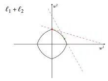
The norm (see also Norms) can be used to approximate the optimal norm via convex relaxation. It can be shown that the norm induces sparsity. In the case of least squares, this problem is known as LASSO in statistics and basis pursuit in signal processing.

regularization can occasionally produce non-unique solutions. A simple example is provided in the figure when the space of possible solutions lies on a 45 degree line. This can be problematic for certain applications, and is overcome by combining with regularization in elastic net regularization, which takes the following form:
Elastic net regularization tends to have a grouping effect, where correlated input features are assigned equal weights.
Elastic net regularization is commonly used in practice and is implemented in many machine learning libraries.
Proximal methods
While the norm does not result in an NP-hard problem, the norm is convex but is not strictly differentiable due to the kink at x = 0. Subgradient methods which rely on the subderivative can be used to solve regularized learning problems. However, faster convergence can be achieved through proximal methods.
For a problem such that is convex, continuous, differentiable, with Lipschitz continuous gradient (such as the least squares loss function), and is convex, continuous, and proper, then the proximal method to solve the problem is as follows. First define the proximal operator
and then iterate
The proximal method iteratively performs gradient descent and then projects the result back into the space permitted by .
When is the regularizer, the proximal operator is equivalent to the soft-thresholding operator,
This allows for efficient computation.
Group sparsity without overlaps
Groups of features can be regularized by a sparsity constraint, which can be useful for expressing certain prior knowledge into an optimization problem.
In the case of a linear model with non-overlapping known groups, a regularizer can be defined:
- where
This can be viewed as inducing a regularizer over the norm over members of each group followed by an norm over groups.
This can be solved by the proximal method, where the proximal operator is a block-wise soft-thresholding function:
Group sparsity with overlaps
The algorithm described for group sparsity without overlaps can be applied to the case where groups do overlap, in certain situations. This will likely result in some groups with all zero elements, and other groups with some non-zero and some zero elements.
If it is desired to preserve the group structure, a new regularizer can be defined:
For each , is defined as the vector such that the restriction of to the group equals and all other entries of are zero. The regularizer finds the optimal disintegration of into parts. It can be viewed as duplicating all elements that exist in multiple groups. Learning problems with this regularizer can also be solved with the proximal method with a complication. The proximal operator cannot be computed in closed form, but can be effectively solved iteratively, inducing an inner iteration within the proximal method iteration.
Regularizers for semi-supervised learning
When labels are more expensive to gather than input examples, semi-supervised learning can be useful. Regularizers have been designed to guide learning algorithms to learn models that respect the structure of unsupervised training samples. If a symmetric weight matrix is given, a regularizer can be defined:
If encodes the result of some distance metric for points and , it is desirable that . This regularizer captures this intuition, and is equivalent to:
- where is the Laplacian matrix of the graph induced by .
The optimization problem can be solved analytically if the constraint is applied for all supervised samples. The labeled part of the vector is therefore obvious. The unlabeled part of is solved for by:
The pseudo-inverse can be taken because has the same range as .
Regularizers for multitask learning
In the case of multitask learning, problems are considered simultaneously, each related in some way. The goal is to learn functions, ideally borrowing strength from the relatedness of tasks, that have predictive power. This is equivalent to learning the matrix .
Sparse regularizer on columns
This regularizer defines an L2 norm on each column and an L1 norm over all columns. It can be solved by proximal methods.
Nuclear norm regularization
- where is the eigenvalues in the singular value decomposition of .
Mean-constrained regularization
This regularizer constrains the functions learned for each task to be similar to the overall average of the functions across all tasks. This is useful for expressing prior information that each task is expected to share with each other task. An example is predicting blood iron levels measured at different times of the day, where each task represents an individual.
Clustered mean-constrained regularization
- where is a cluster of tasks.
This regularizer is similar to the mean-constrained regularizer, but instead enforces similarity between tasks within the same cluster. This can capture more complex prior information. This technique has been used to predict Netflix recommendations. A cluster would correspond to a group of people who share similar preferences.
Graph-based similarity
More generally than above, similarity between tasks can be defined by a function. The regularizer encourages the model to learn similar functions for similar tasks.
- for a given symmetric similarity matrix .
Other uses of regularization in statistics and machine learning
Bayesian learning methods make use of a prior probability that (usually) gives lower probability to more complex models. Well-known model selection techniques include the Akaike information criterion (AIC), minimum description length (MDL), and the Bayesian information criterion (BIC). Alternative methods of controlling overfitting not involving regularization include cross-validation.
Examples of applications of different methods of regularization to the linear model are:
| Model | Fit measure | Entropy measure[4][7] |
|---|---|---|
| AIC/BIC | ||
| Ridge regression[8] | ||
| Lasso[9] | ||
| Basis pursuit denoising | ||
| Rudin–Osher–Fatemi model (TV) | ||
| Potts model | ||
| RLAD[10] | ||
| Dantzig Selector[11] | ||
| SLOPE[12] |
See also
Notes
-
Kratsios, Anastasis (2020). "Deep Arbitrage-Free Learning in a Generalized HJM Framework via Arbitrage-Regularization Data". Risks. 8 (2): . doi:10.3390/risks8020040.
Term structure models can be regularized to remove arbitrage opportunities [sic?].
{{cite journal}}: Cite journal requires|journal=(help) - Bühlmann, Peter; Van De Geer, Sara (2011). Statistics for High-Dimensional Data. Springer Series in Statistics. p. 9. doi:10.1007/978-3-642-20192-9. ISBN 978-3-642-20191-2.
If p > n, the ordinary least squares estimator is not unique and will heavily overfit the data. Thus, a form of complexity regularization will be necessary.
- "Deep Learning Book". www.deeplearningbook.org. Retrieved 2021-01-29.
- Bishop, Christopher M. (2007). Pattern recognition and machine learning (Corr. printing. ed.). New York: Springer. ISBN 978-0-387-31073-2.
- For the connection between maximum a posteriori estimation and ridge regression, see Weinberger, Kilian (July 11, 2018). "Linear / Ridge Regression". CS4780 Machine Learning Lecture 13. Cornell.
- Natarajan, B. (1995-04-01). "Sparse Approximate Solutions to Linear Systems". SIAM Journal on Computing. 24 (2): 227–234. doi:10.1137/S0097539792240406. ISSN 0097-5397. S2CID 2072045.
- Duda, Richard O. (2004). Pattern classification + computer manual : hardcover set (2. ed.). New York [u.a.]: Wiley. ISBN 978-0-471-70350-1.
- Arthur E. Hoerl; Robert W. Kennard (1970). "Ridge regression: Biased estimation for nonorthogonal problems". Technometrics. 12 (1): 55–67. doi:10.2307/1267351. JSTOR 1267351.
- Tibshirani, Robert (1996). "Regression Shrinkage and Selection via the Lasso" (PostScript). Journal of the Royal Statistical Society, Series B. 58 (1): 267–288. MR 1379242. Retrieved 2009-03-19.
- Li Wang, Michael D. Gordon & Ji Zhu (2006). "Regularized Least Absolute Deviations Regression and an Efficient Algorithm for Parameter Tuning". Sixth International Conference on Data Mining. pp. 690–700. doi:10.1109/ICDM.2006.134. ISBN 978-0-7695-2701-7.
- Candes, Emmanuel; Tao, Terence (2007). "The Dantzig selector: Statistical estimation when p is much larger than n". Annals of Statistics. 35 (6): 2313–2351. arXiv:math/0506081. doi:10.1214/009053606000001523. MR 2382644. S2CID 88524200.
-
Małgorzata Bogdan, Ewout van den Berg, Weijie Su & Emmanuel J. Candes (2013). "Statistical estimation and testing via the ordered L1 norm". arXiv:1310.1969 [stat.ME].
{{cite arXiv}}: CS1 maint: multiple names: authors list (link)
References
- Neumaier, A. (1998). "Solving ill-conditioned and singular linear systems: A tutorial on regularization" (PDF). SIAM Review. 40 (3): 636–666. Bibcode:1998SIAMR..40..636N. doi:10.1137/S0036144597321909.