Shot transition detection
Shot transition detection (or simply shot detection) also called cut detection is a field of research of video processing. Its subject is the automated detection of transitions between shots in digital video with the purpose of temporal segmentation of videos.[1]
Use
Shot transition detection is used to split up a film into basic temporal units called shots; a shot is a series of interrelated consecutive pictures taken contiguously by a single camera and representing a continuous action in time and space.[2]
This operation is of great use in software for post-production of videos. It is also a fundamental step of automated indexing and content-based video retrieval or summarization applications which provide an efficient access to huge video archives, e.g. an application may choose a representative picture from each scene to create a visual overview of the whole film and, by processing such indexes, a search engine can process search items like "show me all films where there's a scene with a lion in it."
Cut detection can do nothing that a human editor couldn't do manually, however it is advantageous as it saves time. Furthermore, due to the increase in the use of digital video and, consequently, in the importance of the aforementioned indexing applications, the automatic cut detection is very important nowadays.
Basic technical terms


In simple terms cut detection is about finding the positions in a video in that one scene is replaced by another one with different visual content. Technically speaking the following terms are used:
A digital video consists of frames that are presented to the viewer's eye in rapid succession to create the impression of movement. "Digital" in this context means both that a single frame consists of pixels and the data is present as binary data, such that it can be processed with a computer. Each frame within a digital video can be uniquely identified by its frame index, a serial number.
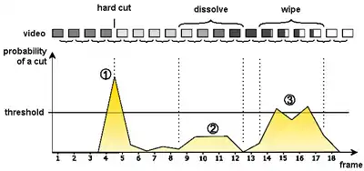
A shot is a sequence of frames shot uninterruptedly by one camera. There are several film transitions usually used in film editing to juxtapose adjacent shots; In the context of shot transition detection they are usually group into two types:[3]
- Abrupt Transitions - This is a sudden transition from one shot to another, i. e. one frame belongs to the first shot, the next frame belongs to the second shot. They are also known as hard cuts or simply cuts.
- Gradual Transitions - In this kind of transitions the two shots are combined using chromatic, spatial or spatial-chromatic effects which gradually replace one shot by another. These are also often known as soft transitions and can be of various types, e.g., wipes, dissolves, fades...
"Detecting a cut" means that the position of a cut is gained; more precisely a hard cut is gained as "hard cut between frame i and frame i+1", a soft cut as "soft cut from frame i to frame j".
A transition that is detected correctly is called a hit, a cut that is there but was not detected is called a missed hit and a position in that the software assumes a cut, but where actually no cut is present, is called a false hit.
An introduction to film editing and an exhaustive list of shot transition techniques can be found at film editing.
Vastness of the problem
Although cut detection appears to be a simple task for a human being, it is a non-trivial task for computers. Cut detection would be a trivial problem if each frame of a video was enriched with additional information about when and by which camera it was taken. Possibly no algorithm for cut detection will ever be able to detect all cuts with certainty, unless it is provided with powerful artificial intelligence.
While most algorithms achieve good results with hard cuts, many fail with recognizing soft cuts. Hard cuts usually go together with sudden and extensive changes in the visual content while soft cuts feature slow and gradual changes. A human being can compensate this lack of visual diversity with understanding the meaning of a scene. While a computer assumes a black line wiping a shot away to be "just another regular object moving slowly through the on-going scene", a person understands that the scene ends and is replaced by a black screen.
Methods
Each method for cut detection works on a two-phase-principle:
- Scoring – Each pair of consecutive frames of a digital video is given a certain score that represents the similarity/dissimilarity between them.
- Decision – All scores calculated previously are evaluated and a cut is detected if the score is considered high.
This principle is error prone. First, because even minor exceedings of the threshold value produce a hit, it must be ensured that phase one scatters values widely to maximize the average difference between the score for "cut" and "no cut". Second, the threshold must be chosen with care; usually useful values can be gained with statistical methods.

Scoring
There are many possible scores used to access the differences in the visual content; some of the most common are:
- Sum of absolute differences (SAD). This is both the most obvious and most simple algorithm of all: The two consecutive frames are compared pixel by pixel, summing up the absolute values of the differences of each two corresponding pixels. The result is a positive number that is used as the score. SAD reacts very sensitively to even minor changes within a scene: fast movements of the camera, explosions or the simple switching on of a light in a previously dark scene result in false hits. On the other hand, SAD hardly reacts to soft cuts at all. Yet, SAD is used often to produce a basic set of "possible hits" as it detects all visible hard cuts with utmost probability.
- Histogram differences (HD). Histogram differences is very similar to Sum of absolute differences. The difference is that HD computes the difference between the histograms of two consecutive frames; a histogram is a table that contains for each color within a frame the number of pixels that are shaded in that color. HD is not as sensitive to minor changes within a scene as SAD and thus produces less false hits. One major problem of HD is that two images can have exactly the same histograms while the shown content differs extremely, e. g. a picture of the sea and a beach can have the same histogram as one of a corn field and the sky. HD offers no guarantee that it recognizes hard cuts.
- Edge change ratio (ECR). The ECR attempts to compare the actual content of two frames. It transforms both frames to edge pictures, i. e. it extracts the probable outlines of objects within the pictures (see edge detection for details). Afterwards it compares these edge pictures using dilation to compute a probability that the second frame contains the same objects as the first frame. The ECR is one of the best performing algorithms for scoring. It reacts very sensitively to hard cuts and can detect many soft cuts by nature. In its basic form even ECR cannot detect soft cuts such as wipes as it considers the fading-in objects as regular objects moving through the scene. Yet, ECR can be extended manually to recognize special forms of soft cuts.
Finally, a combination of two or more of these scores can improve the performance.
Decision
In the decision phase the following approaches are usually used:
- Fixed Threshold – In this approach, the scores are compared to a threshold which was set previously and if the score is higher than the threshold a cut is declared.
- Adaptive Threshold – In this approach, the scores are compared to a threshold which considers various scores in the video to adapt the threshold to the properties of the current video. Like in the previous case, if the score is higher than the corresponding threshold a cut is declared.
- Machine Learning - Machine learning techniques can be applied also to the decision process.
Cost
All of the above algorithms complete in O(n) — that is to say they run in linear time — where n is the number of frames in the input video. The algorithms differ in a constant factor that is determined mostly by the image resolution of the video.
Measures for quality
Usually the following three measures are used to measure the quality of a cut detection algorithm:
- Recall is the probability that an existing cut will be detected:
- Precision is the probability that an assumed cut is in fact a cut:
- F1 is a combined measure that results in high value if, and only if, both precision and recall result in high values:
The symbols stand for: C, the number of correctly detected cuts ("correct hits"), M, the number of not detected cuts ("missed hits") and F, the number of falsely detected cuts ("false hits"). All of these measures are mathematical measures, i. e. they deliver values in between 0 and 1. The basic rule is: the higher the value, the better performs the algorithm.
Benchmarks
| Benchmark | Videos | Hours | Frames | Shot transitions | Participants | Years |
|---|---|---|---|---|---|---|
| TRECVid | 12 - 42 | 4.8 - 7.5 | 545,068 - 744,604 | 2090 - 4806 | 57 | 2001 - 2007 |
| MSU SBD | 31 | 21.45 | 1,900,000+ | 10883 | 7 | 2020 - 2021 |
TRECVid SBD Benchmark 2001-2007[4]
Automatic shot transition detection was one of the tracks of activity within the annual TRECVid benchmarking exercise from 2001 to 2007. There were 57 algorithms from different research groups. Сalculations of F score were performed for each algorithm on a dataset, which was replenished annually.
| Group | F score | Processing speed (compared to real-time) | Open source | Used metrics and technologies |
|---|---|---|---|---|
| Tsinghua U.[5] | 0.897 | ×0.23 | No | Mean of Pixel Intensities Standard Deviation of Pixel Intensities Color Histogram Pixel-wise Difference Motion Vector |
| NICTA[6] | 0.892 | ×2.30 | No | Machine learning |
| IBM Research[7] | 0.876 | ×0.30 | No | Color histogram Localized Edges direction histogram Gray-level Thumbnails comparison Frame luminance |
MSU SBD Benchmark 2020-2021 [8]
The benchmark has compared 6 methods on more than 120 videos from RAI and MSU CC datasets with different types of scene changes, some of which were added manually.[9] The authors state that the main feature of this benchmark is the complexity of shot transitions in the dataset. To prove it they calculate SI/TI metric of shots and compare it with others publicly available datasets.
| Algorithm | F score | Processing speed (FPS) | Open source | Used metrics and technologies |
|---|---|---|---|---|
| Saeid Dadkhah[10] | 0.797 | 86 | Yes | Color histogram Adaptive threshold |
| Max Reimann[11] | 0.787 | 76 | Yes | SVM for cuts Neural networks for graduals transitions Color Histogram |
| VQMT[12] | 0.777 | 308 | No | Edges histograms Motion compensation Color histograms |
| PySceneDetect[13] | 0.776 | 321 | Yes | Frame intensity |
| FFmpeg[14] | 0.772 | 165 | Yes | Color histogram |
References
- P. Balasubramaniam; R Uthayakumar (2 March 2012). Mathematical Modelling and Scientific Computation: International Conference, ICMMSC 2012, Gandhigram, Tamil Nadu, India, March 16-18, 2012. Springer. pp. 421–. ISBN 978-3-642-28926-2.
- Weiming Shen; Jianming Yong; Yun Yang (18 December 2008). Computer Supported Cooperative Work in Design IV: 11th International Conference, CSCWD 2007, Melbourne, Australia, April 26-28, 2007. Revised Selected Papers. Springer Science & Business Media. pp. 100–. ISBN 978-3-540-92718-1.
- Joan Cabestany; Ignacio Rojas; Gonzalo Joya (30 May 2011). Advances in Computational Intelligence: 11th International Work-Conference on Artificial Neural Networks, IWANN 2011, Torremolinos-Málaga, Spain, June 8-10, 2011, Proceedings. Springer Science & Business Media. pp. 521–. ISBN 978-3-642-21500-1.
Shot detection is performed by means of shot transition detection algorithms. Two different types of transitions are used to split a video into shots: – Abrupt transitions, also referred as cuts or straight cuts, occur when a sudden change from one ...
- Smeaton, A. F., Over, P., & Doherty, A. R. (2010). Video shot boundary detection: Seven years of TRECVid activity. Computer Vision and Image Understanding, 114(4), 411–418. doi:10.1016/j.cviu.2009.03.011
- Yuan, J., Zheng, W., Chen, L., Ding, D., Wang, D., Tong, Z., Wang, H., Wu, J., Li, J., Lin, F., & Zhang, B. (2004). Tsinghua University at TRECVID 2004: Shot Boundary Detection and High-Level Feature Extraction. TRECVID.
- Yu, Zhenghua, S. Vishwanathan and Alex Smola. “NICTA at TRECVID 2005 Shot Boundary Detection Task.” TRECVID (2005).
- A. Amir, The IBM Shot Boundary Detection System at TRECVID 2003, in: TRECVID 2005 Workshop Notebook Papers, National Institute of Standards and Technology, MD, USA, 2003.
- "MSU SBD Benchmark 2020". Archived from the original on 2021-02-13. Retrieved 2021-02-19.
- "MSU SBD Benchmark 2020". Archived from the original on 2021-02-13. Retrieved 2021-02-19.
- "SaeidDadkhah/Shot-Boundary-Detection". GitHub. 19 September 2021.
- "Shot-Boundary-Detection". GitHub. 11 September 2021.
- "MSU Scene Change Detector (SCD)".
- "Home - PySceneDetect".
- "Ffprobe Documentation".