Autoencoder
An autoencoder is a type of artificial neural network used to learn efficient codings of unlabeled data (unsupervised learning).[1][2] An autoencoder learns two functions: an encoding function that transforms the input data, and a decoding function that recreates the input data from the encoded representation. The autoencoder learns an efficient representation (encoding) for a set of data, typically for dimensionality reduction.
| Part of a series on |
| Machine learning and data mining |
|---|
 |
Variants exist, aiming to force the learned representations to assume useful properties.[3] Examples are regularized autoencoders (Sparse, Denoising and Contractive), which are effective in learning representations for subsequent classification tasks,[4] and Variational autoencoders, with applications as generative models.[5] Autoencoders are applied to many problems, including facial recognition,[6] feature detection,[7] anomaly detection and acquiring the meaning of words.[8][9] Autoencoders are also generative models which can randomly generate new data that is similar to the input data (training data).[7]
Mathematical principles
Definition
An autoencoder is defined by the following components:
Two sets: the space of decoded messages ; the space of encoded messages . Almost always, both and are Euclidean spaces, that is, for some .
Two parametrized families of functions: the encoder family , parametrized by ; the decoder family , parametrized by .
For any , we usually write , and refer to it as the code, the latent variable, latent representation, latent vector, etc. Conversely, for any , we usually write , and refer to it as the (decoded) message.
Usually, both the encoder and the decoder are defined as multilayer perceptrons. For example, a one-layer-MLP encoder is:
where is an element-wise activation function such as a sigmoid function or a rectified linear unit, is a matrix called "weight", and is a vector called "bias".
Training an autoencoder
An autoencoder, by itself, is simply a tuple of two functions. To judge its quality, we need a task. A task is defined by a reference probability distribution over , and a "reconstruction quality" function , such that measures how much differs from .
With those, we can define the loss function for the autoencoder as
The optimal autoencoder for the given task is then . The search for the optimal autoencoder can be accomplished by any mathematical optimization technique, but usually by gradient descent. This search process is referred to as "training the autoencoder". In most situations, the reference distribution is just the empirical distribution given by a dataset , so that
where and is the Dirac measure, and the quality function is just L2 loss: . Then the problem of searching for the optimal autoencoder is just a least-squares optimization:
Interpretation
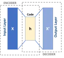
An autoencoder has two main parts: an encoder that maps the message to a code, and a decoder that reconstructs the message from the code. An optimal autoencoder would perform as close to perfect reconstruction as possible, with "close to perfect" defined by the reconstruction quality function .
The simplest way to perform the copying task perfectly would be to duplicate the signal. To suppress this behavior, the code space usually has fewer dimensions than the message space .
Such an autoencoder is called undercomplete. It can be interpreted as compressing the message, or reducing its dimensionality.[1][10]
At the limit of an ideal undercomplete autoencoder, every possible code in the code space is used to encode a message that really appears in the distribution , and the decoder is also perfect: . This ideal autoencoder can then be used to generate messages indistinguishable from real messages, by feeding its decoder arbitrary code and obtaining , which is a message that really appears in the distribution .
If the code space has dimension larger than (overcomplete), or equal to, the message space , or the hidden units are given enough capacity, an autoencoder can learn the identity function and become useless. However, experimental results found that overcomplete autoencoders might still learn useful features.[11]
In the ideal setting, the code dimension and the model capacity could be set on the basis of the complexity of the data distribution to be modeled. A standard way to do so is to add modifications to the basic autoencoder, to be detailed below.[3]
History
The autoencoder was first proposed as a nonlinear generalization of principal components analysis (PCA) by Kramer.[1] The autoencoder has also been called the autoassociator,[12] or Diabolo network.[13][11] Its first applications date to early 1990s.[3][14][15] Their most traditional application was dimensionality reduction or feature learning, but the concept became widely used for learning generative models of data.[16][17] Some of the most powerful AIs in the 2010s involved autoencoders stacked inside deep neural networks.[18]
Variations
Regularized autoencoders
Various techniques exist to prevent autoencoders from learning the identity function and to improve their ability to capture important information and learn richer representations.
Sparse autoencoder (SAE)
Inspired by the sparse coding hypothesis in neuroscience, sparse autoencoders are variants of autoencoders, such that the codes for messages tend to be sparse codes, that is, is close to zero in most entries. Sparse autoencoders may include more (rather than fewer) hidden units than inputs, but only a small number of the hidden units are allowed to be active at the same time.[18] Encouraging sparsity improves performance on classification tasks.[19]
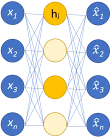
There are two main ways to enforce sparsity. One way is to simply clamp all but the highest-k activations of the latent code to zero. This is the k-sparse autoencoder.[20]
The k-sparse autoencoder inserts the following "k-sparse function" in the latent layer of a standard autoencoder:
where if ranks in the top k, and 0 otherwise.
Backpropagating through is simple: set gradient to 0 for entries, and keep gradient for entries. This is essentially a generalized ReLU function.[20]
The other way is a relaxed version of the k-sparse autoencoder. Instead of forcing sparsity, we add a sparsity regularization loss, then optimize for
where measures how much sparsity we want to enforce.[21]
Let the autoencoder architecture have layers. To define a sparsity regularization loss, we need a "desired" sparsity for each layer, a weight for how much to enforce each sparsity, and a function to measure how much two sparsities differ.
For each input , let the actual sparsity of activation in each layer be
where is the activation in the -th neuron of the -th layer upon input . The sparsity loss upon input for one layer is , and the sparsity regularization loss for the entire autoencoder is the expected weighted sum of sparsity losses:
Typically, the function is either the Kullback-Leibler (KL) divergence, as[19][21][22][23]
or the L1 loss, as , or the L2 loss, as .
Alternatively, the sparsity regularization loss may be defined without reference to any "desired sparsity", but simply force as much sparsity as possible. In this case, one can sparsity regularization loss as
where is the activation vector in the -th layer of the autoencoder. The norm is usually the L1 norm (giving the L1 sparse autoencoder) or the L2 norm (giving the L2 sparse autoencoder).
Denoising autoencoder (DAE)
Denoising autoencoders (DAE) try to achieve a good representation by changing the reconstruction criterion.[3][4]
A DAE is defined by adding a noise process to the standard autoencoder. A noise process is defined by a probability distribution over functions . That is, the function takes a message , and corrupts it to a noisy version . The function is selected randomly, with a probability distribution .
Given a task , the problem of training a DAE is the optimization problem:
That is, the optimal DAE should take any noisy message and attempt to recover the original message without noise, thus the name "denoising".
Usually, the noise process is applied only during training and testing, not during downstream use.
The use of DAE depends on two assumptions:
- There exist representations to the messages that are relatively stable and robust to the type of noise we are likely to encounter;
- The said representations capture structures in the input distribution that are useful for our purposes.[4]
Example noise processes include:
- additive isotropic Gaussian noise,
- masking noise (a fraction of the input is randomly chosen and set to 0)
- salt-and-pepper noise (a fraction of the input is randomly chosen and randomly set to its minimum or maximum value).[4]
Contractive autoencoder (CAE)
A contractive autoencoder adds the contractive regularization loss to the standard autoencoder loss:
where measures how much contractive-ness we want to enforce. The contractive regularization loss itself is defined as the expected Frobenius norm of the Jacobian matrix of the encoder activations with respect to the input:
To understand what measures, note the fact
for any message , and small variation in it. Thus, if is small, it means that a small neighborhood of the message maps to a small neighborhood of its code. This is a desired property, as it means small variation in the message leads to small, perhaps even zero, variation in its code, like how two pictures may look the same even if they are not exactly the same.
The DAE can be understood as an infinitesimal limit of CAE: in the limit of small Gaussian input noise, DAEs make the reconstruction function resist small but finite-sized input perturbations, while CAEs make the extracted features resist infinitesimal input perturbations.
Minimal description length autoencoder
Concrete autoencoder
The concrete autoencoder is designed for discrete feature selection.[25] A concrete autoencoder forces the latent space to consist only of a user-specified number of features. The concrete autoencoder uses a continuous relaxation of the categorical distribution to allow gradients to pass through the feature selector layer, which makes it possible to use standard backpropagation to learn an optimal subset of input features that minimize reconstruction loss.
Variational autoencoder (VAE)
Variational autoencoders (VAEs) belong to the families of variational Bayesian methods. Despite the architectural similarities with basic autoencoders, VAEs are architecture with different goals and with a completely different mathematical formulation. The latent space is in this case composed by a mixture of distributions instead of a fixed vector.
Given an input dataset characterized by an unknown probability function and a multivariate latent encoding vector , the objective is to model the data as a distribution , with defined as the set of the network parameters so that .
Advantages of depth
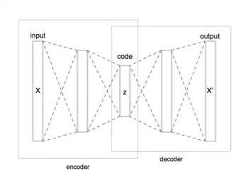
Autoencoders are often trained with a single-layer encoder and a single-layer decoder, but using many-layered (deep) encoders and decoders offers many advantages.[3]
- Depth can exponentially reduce the computational cost of representing some functions.
- Depth can exponentially decrease the amount of training data needed to learn some functions.
- Experimentally, deep autoencoders yield better compression compared to shallow or linear autoencoders.[10]
Training
Geoffrey Hinton developed the deep belief network technique for training many-layered deep autoencoders. His method involves treating each neighboring set of two layers as a restricted Boltzmann machine so that pretraining approximates a good solution, then using backpropagation to fine-tune the results.[10]
Researchers have debated whether joint training (i.e. training the whole architecture together with a single global reconstruction objective to optimize) would be better for deep auto-encoders.[26] A 2015 study showed that joint training learns better data models along with more representative features for classification as compared to the layerwise method.[26] However, their experiments showed that the success of joint training depends heavily on the regularization strategies adopted.[26][27]
Applications
The two main applications of autoencoders are dimensionality reduction and information retrieval,[3] but modern variations have been applied to other tasks.
Dimensionality reduction
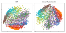
Dimensionality reduction was one of the first deep learning applications.[3]
For Hinton's 2006 study,[10] he pretrained a multi-layer autoencoder with a stack of RBMs and then used their weights to initialize a deep autoencoder with gradually smaller hidden layers until hitting a bottleneck of 30 neurons. The resulting 30 dimensions of the code yielded a smaller reconstruction error compared to the first 30 components of a principal component analysis (PCA), and learned a representation that was qualitatively easier to interpret, clearly separating data clusters.[3][10]
Representing dimensions can improve performance on tasks such as classification.[3] Indeed, the hallmark of dimensionality reduction is to place semantically related examples near each other.[29]
Principal component analysis
If linear activations are used, or only a single sigmoid hidden layer, then the optimal solution to an autoencoder is strongly related to principal component analysis (PCA).[30][31] The weights of an autoencoder with a single hidden layer of size (where is less than the size of the input) span the same vector subspace as the one spanned by the first principal components, and the output of the autoencoder is an orthogonal projection onto this subspace. The autoencoder weights are not equal to the principal components, and are generally not orthogonal, yet the principal components may be recovered from them using the singular value decomposition.[32]
However, the potential of autoencoders resides in their non-linearity, allowing the model to learn more powerful generalizations compared to PCA, and to reconstruct the input with significantly lower information loss.[10]
Information retrieval and Search engine optimization
Information retrieval benefits particularly from dimensionality reduction in that search can become more efficient in certain kinds of low dimensional spaces. Autoencoders were indeed applied to semantic hashing, proposed by Salakhutdinov and Hinton in 2007.[29] By training the algorithm to produce a low-dimensional binary code, all database entries could be stored in a hash table mapping binary code vectors to entries. This table would then support information retrieval by returning all entries with the same binary code as the query, or slightly less similar entries by flipping some bits from the query encoding.
The encoder-decoder architecture, often used in natural language processing and neural networks, can be scientifically applied in the field of SEO (Search Engine Optimization) in various ways:
- Text Processing: By using an autoencoder, it's possible to compress the text of web pages into a more compact vector representation. This can help reduce page loading times and improve indexing by search engines.
- Noise Reduction: Autoencoders can be used to remove noise from the textual data of web pages. This can lead to a better understanding of the content by search engines, thereby enhancing ranking in search engine result pages.
- Meta Tag and Snippet Generation: Autoencoders can be trained to automatically generate meta tags, snippets, and descriptions for web pages using the page content. This can optimize the presentation in search results, increasing the Click-Through Rate (CTR).
- Content Clustering: Using an autoencoder, web pages with similar content can be automatically grouped together. This can help organize the website logically and improve navigation, potentially positively affecting user experience and search engine rankings.
- Generation of Related Content: An autoencoder can be employed to generate content related to what is already present on the site. This can enhance the website's attractiveness to search engines and provide users with additional relevant information.
- Keyword Detection: Autoencoders can be trained to identify keywords and important concepts within the content of web pages. This can assist in optimizing keyword usage for better indexing.
- Semantic Search: By using autoencoder techniques, semantic representation models of content can be created. These models can be used to enhance search engines' understanding of the themes covered in web pages.
In essence, the encoder-decoder architecture or autoencoders can be leveraged in SEO to optimize web page content, improve their indexing, and enhance their appeal to both search engines and users.
Anomaly detection
Another application for autoencoders is anomaly detection.[2][33][34][35][36][37] By learning to replicate the most salient features in the training data under some of the constraints described previously, the model is encouraged to learn to precisely reproduce the most frequently observed characteristics. When facing anomalies, the model should worsen its reconstruction performance. In most cases, only data with normal instances are used to train the autoencoder; in others, the frequency of anomalies is small compared to the observation set so that its contribution to the learned representation could be ignored. After training, the autoencoder will accurately reconstruct "normal" data, while failing to do so with unfamiliar anomalous data.[35] Reconstruction error (the error between the original data and its low dimensional reconstruction) is used as an anomaly score to detect anomalies.[35]
Recent literature has however shown that certain autoencoding models can, counterintuitively, be very good at reconstructing anomalous examples and consequently not able to reliably perform anomaly detection.[38][39]
Image processing
The characteristics of autoencoders are useful in image processing.
One example can be found in lossy image compression, where autoencoders outperformed other approaches and proved competitive against JPEG 2000.[40][41]
Another useful application of autoencoders in image preprocessing is image denoising.[42][43][44]
Autoencoders found use in more demanding contexts such as medical imaging where they have been used for image denoising[45] as well as super-resolution.[46][47] In image-assisted diagnosis, experiments have applied autoencoders for breast cancer detection[48] and for modelling the relation between the cognitive decline of Alzheimer's disease and the latent features of an autoencoder trained with MRI.[49]
Drug discovery
In 2019 molecules generated with variational autoencoders were validated experimentally in mice.[50][51]
Popularity prediction
Recently, a stacked autoencoder framework produced promising results in predicting popularity of social media posts,[52] which is helpful for online advertising strategies.
Machine translation
Autoencoders have been applied to machine translation, which is usually referred to as neural machine translation (NMT).[53][54] Unlike traditional autoencoders, the output does not match the input - it is in another language. In NMT, texts are treated as sequences to be encoded into the learning procedure, while on the decoder side sequences in the target language(s) are generated. Language-specific autoencoders incorporate further linguistic features into the learning procedure, such as Chinese decomposition features.[55] Machine translation is rarely still done with autoencoders, due to the availability of more effective transformer networks.
References
- Kramer, Mark A. (1991). "Nonlinear principal component analysis using autoassociative neural networks" (PDF). AIChE Journal. 37 (2): 233–243. doi:10.1002/aic.690370209.
- Kramer, M. A. (1992-04-01). "Autoassociative neural networks". Computers & Chemical Engineering. Neutral network applications in chemical engineering. 16 (4): 313–328. doi:10.1016/0098-1354(92)80051-A. ISSN 0098-1354.
- Goodfellow, Ian; Bengio, Yoshua; Courville, Aaron (2016). Deep Learning. MIT Press. ISBN 978-0262035613.
- Vincent, Pascal; Larochelle, Hugo (2010). "Stacked Denoising Autoencoders: Learning Useful Representations in a Deep Network with a Local Denoising Criterion". Journal of Machine Learning Research. 11: 3371–3408.
- Welling, Max; Kingma, Diederik P. (2019). "An Introduction to Variational Autoencoders". Foundations and Trends in Machine Learning. 12 (4): 307–392. arXiv:1906.02691. Bibcode:2019arXiv190602691K. doi:10.1561/2200000056. S2CID 174802445.
- Hinton GE, Krizhevsky A, Wang SD. Transforming auto-encoders. In International Conference on Artificial Neural Networks 2011 Jun 14 (pp. 44-51). Springer, Berlin, Heidelberg.
- Géron, Aurélien (2019). Hands-On Machine Learning with Scikit-Learn, Keras, and TensorFlow. Canada: O’Reilly Media, Inc. pp. 739–740.
- Liou, Cheng-Yuan; Huang, Jau-Chi; Yang, Wen-Chie (2008). "Modeling word perception using the Elman network". Neurocomputing. 71 (16–18): 3150. doi:10.1016/j.neucom.2008.04.030.
- Liou, Cheng-Yuan; Cheng, Wei-Chen; Liou, Jiun-Wei; Liou, Daw-Ran (2014). "Autoencoder for words". Neurocomputing. 139: 84–96. doi:10.1016/j.neucom.2013.09.055.
- Hinton, G. E.; Salakhutdinov, R.R. (2006-07-28). "Reducing the Dimensionality of Data with Neural Networks". Science. 313 (5786): 504–507. Bibcode:2006Sci...313..504H. doi:10.1126/science.1127647. PMID 16873662. S2CID 1658773.
- Bengio, Y. (2009). "Learning Deep Architectures for AI" (PDF). Foundations and Trends in Machine Learning. 2 (8): 1795–7. CiteSeerX 10.1.1.701.9550. doi:10.1561/2200000006. PMID 23946944. S2CID 207178999.
- Japkowicz, Nathalie; Hanson, Stephen José; Gluck, Mark A. (2000-03-01). "Nonlinear Autoassociation Is Not Equivalent to PCA". Neural Computation. 12 (3): 531–545. doi:10.1162/089976600300015691. ISSN 0899-7667. PMID 10769321. S2CID 18490972.
- Schwenk, Holger; Bengio, Yoshua (1997). "Training Methods for Adaptive Boosting of Neural Networks". Advances in Neural Information Processing Systems. MIT Press. 10.
- Schmidhuber, Jürgen (January 2015). "Deep learning in neural networks: An overview". Neural Networks. 61: 85–117. arXiv:1404.7828. doi:10.1016/j.neunet.2014.09.003. PMID 25462637. S2CID 11715509.
- Hinton, G. E., & Zemel, R. S. (1994). Autoencoders, minimum description length and Helmholtz free energy. In Advances in neural information processing systems 6 (pp. 3-10).
- Diederik P Kingma; Welling, Max (2013). "Auto-Encoding Variational Bayes". arXiv:1312.6114 [stat.ML].
- Generating Faces with Torch, Boesen A., Larsen L. and Sonderby S.K., 2015 torch
.ch /blog /2015 /11 /13 /gan .html - Domingos, Pedro (2015). "4". The Master Algorithm: How the Quest for the Ultimate Learning Machine Will Remake Our World. Basic Books. "Deeper into the Brain" subsection. ISBN 978-046506192-1.
- Frey, Brendan; Makhzani, Alireza (2013-12-19). "k-Sparse Autoencoders". arXiv:1312.5663. Bibcode:2013arXiv1312.5663M.
{{cite journal}}: Cite journal requires|journal=(help) - Makhzani, Alireza; Frey, Brendan (2013). "K-Sparse Autoencoders". arXiv:1312.5663 [cs.LG].
- Ng, A. (2011). Sparse autoencoder. CS294A Lecture notes, 72(2011), 1-19.
- Nair, Vinod; Hinton, Geoffrey E. (2009). "3D Object Recognition with Deep Belief Nets". Proceedings of the 22nd International Conference on Neural Information Processing Systems. NIPS'09. USA: Curran Associates Inc.: 1339–1347. ISBN 9781615679119.
- Zeng, Nianyin; Zhang, Hong; Song, Baoye; Liu, Weibo; Li, Yurong; Dobaie, Abdullah M. (2018-01-17). "Facial expression recognition via learning deep sparse autoencoders". Neurocomputing. 273: 643–649. doi:10.1016/j.neucom.2017.08.043. ISSN 0925-2312.
- Hinton, Geoffrey E; Zemel, Richard (1993). "Autoencoders, Minimum Description Length and Helmholtz Free Energy". Advances in Neural Information Processing Systems. Morgan-Kaufmann. 6.
- Abid, Abubakar; Balin, Muhammad Fatih; Zou, James (2019-01-27). "Concrete Autoencoders for Differentiable Feature Selection and Reconstruction". arXiv:1901.09346 [cs.LG].
- Zhou, Yingbo; Arpit, Devansh; Nwogu, Ifeoma; Govindaraju, Venu (2014). "Is Joint Training Better for Deep Auto-Encoders?". arXiv:1405.1380 [stat.ML].
- R. Salakhutdinov and G. E. Hinton, “Deep Boltzmann machines,” in AISTATS, 2009, pp. 448–455.
- "Fashion MNIST". GitHub. 2019-07-12.
- Salakhutdinov, Ruslan; Hinton, Geoffrey (2009-07-01). "Semantic hashing". International Journal of Approximate Reasoning. Special Section on Graphical Models and Information Retrieval. 50 (7): 969–978. doi:10.1016/j.ijar.2008.11.006. ISSN 0888-613X.
- Bourlard, H.; Kamp, Y. (1988). "Auto-association by multilayer perceptrons and singular value decomposition". Biological Cybernetics. 59 (4–5): 291–294. doi:10.1007/BF00332918. PMID 3196773. S2CID 206775335.
- Chicco, Davide; Sadowski, Peter; Baldi, Pierre (2014). "Deep autoencoder neural networks for gene ontology annotation predictions". Proceedings of the 5th ACM Conference on Bioinformatics, Computational Biology, and Health Informatics - BCB '14. p. 533. doi:10.1145/2649387.2649442. hdl:11311/964622. ISBN 9781450328944. S2CID 207217210.
- Plaut, E (2018). "From Principal Subspaces to Principal Components with Linear Autoencoders". arXiv:1804.10253 [stat.ML].
- Morales-Forero, A.; Bassetto, S. (December 2019). "Case Study: A Semi-Supervised Methodology for Anomaly Detection and Diagnosis". 2019 IEEE International Conference on Industrial Engineering and Engineering Management (IEEM). Macao, Macao: IEEE. pp. 1031–1037. doi:10.1109/IEEM44572.2019.8978509. ISBN 978-1-7281-3804-6. S2CID 211027131.
- Sakurada, Mayu; Yairi, Takehisa (December 2014). "Anomaly Detection Using Autoencoders with Nonlinear Dimensionality Reduction". Proceedings of the MLSDA 2014 2nd Workshop on Machine Learning for Sensory Data Analysis. Gold Coast, Australia QLD, Australia: ACM Press. pp. 4–11. doi:10.1145/2689746.2689747. ISBN 978-1-4503-3159-3. S2CID 14613395.
- An, J., & Cho, S. (2015). Variational Autoencoder based Anomaly Detection using Reconstruction Probability. Special Lecture on IE, 2, 1-18.
- Zhou, Chong; Paffenroth, Randy C. (2017-08-04). "Anomaly Detection with Robust Deep Autoencoders". Proceedings of the 23rd ACM SIGKDD International Conference on Knowledge Discovery and Data Mining. ACM. pp. 665–674. doi:10.1145/3097983.3098052. ISBN 978-1-4503-4887-4. S2CID 207557733.
- Ribeiro, Manassés; Lazzaretti, André Eugênio; Lopes, Heitor Silvério (2018). "A study of deep convolutional auto-encoders for anomaly detection in videos". Pattern Recognition Letters. 105: 13–22. Bibcode:2018PaReL.105...13R. doi:10.1016/j.patrec.2017.07.016.
- Nalisnick, Eric; Matsukawa, Akihiro; Teh, Yee Whye; Gorur, Dilan; Lakshminarayanan, Balaji (2019-02-24). "Do Deep Generative Models Know What They Don't Know?". arXiv:1810.09136 [stat.ML].
- Xiao, Zhisheng; Yan, Qing; Amit, Yali (2020). "Likelihood Regret: An Out-of-Distribution Detection Score For Variational Auto-encoder". Advances in Neural Information Processing Systems. 33. arXiv:2003.02977.
- Theis, Lucas; Shi, Wenzhe; Cunningham, Andrew; Huszár, Ferenc (2017). "Lossy Image Compression with Compressive Autoencoders". arXiv:1703.00395 [stat.ML].
- Balle, J; Laparra, V; Simoncelli, EP (April 2017). "End-to-end optimized image compression". International Conference on Learning Representations. arXiv:1611.01704.
- Cho, K. (2013, February). Simple sparsification improves sparse denoising autoencoders in denoising highly corrupted images. In International Conference on Machine Learning (pp. 432-440).
- Cho, Kyunghyun (2013). "Boltzmann Machines and Denoising Autoencoders for Image Denoising". arXiv:1301.3468 [stat.ML].
- Buades, A.; Coll, B.; Morel, J. M. (2005). "A Review of Image Denoising Algorithms, with a New One". Multiscale Modeling & Simulation. 4 (2): 490–530. doi:10.1137/040616024. S2CID 218466166.
- Gondara, Lovedeep (December 2016). "Medical Image Denoising Using Convolutional Denoising Autoencoders". 2016 IEEE 16th International Conference on Data Mining Workshops (ICDMW). Barcelona, Spain: IEEE. pp. 241–246. arXiv:1608.04667. Bibcode:2016arXiv160804667G. doi:10.1109/ICDMW.2016.0041. ISBN 9781509059102. S2CID 14354973.
- Zeng, Kun; Yu, Jun; Wang, Ruxin; Li, Cuihua; Tao, Dacheng (January 2017). "Coupled Deep Autoencoder for Single Image Super-Resolution". IEEE Transactions on Cybernetics. 47 (1): 27–37. doi:10.1109/TCYB.2015.2501373. ISSN 2168-2267. PMID 26625442. S2CID 20787612.
- Tzu-Hsi, Song; Sanchez, Victor; Hesham, EIDaly; Nasir M., Rajpoot (2017). "Hybrid deep autoencoder with Curvature Gaussian for detection of various types of cells in bone marrow trephine biopsy images". 2017 IEEE 14th International Symposium on Biomedical Imaging (ISBI 2017). pp. 1040–1043. doi:10.1109/ISBI.2017.7950694. ISBN 978-1-5090-1172-8. S2CID 7433130.
- Xu, Jun; Xiang, Lei; Liu, Qingshan; Gilmore, Hannah; Wu, Jianzhong; Tang, Jinghai; Madabhushi, Anant (January 2016). "Stacked Sparse Autoencoder (SSAE) for Nuclei Detection on Breast Cancer Histopathology Images". IEEE Transactions on Medical Imaging. 35 (1): 119–130. doi:10.1109/TMI.2015.2458702. PMC 4729702. PMID 26208307.
- Martinez-Murcia, Francisco J.; Ortiz, Andres; Gorriz, Juan M.; Ramirez, Javier; Castillo-Barnes, Diego (2020). "Studying the Manifold Structure of Alzheimer's Disease: A Deep Learning Approach Using Convolutional Autoencoders". IEEE Journal of Biomedical and Health Informatics. 24 (1): 17–26. doi:10.1109/JBHI.2019.2914970. PMID 31217131. S2CID 195187846.
- Zhavoronkov, Alex (2019). "Deep learning enables rapid identification of potent DDR1 kinase inhibitors". Nature Biotechnology. 37 (9): 1038–1040. doi:10.1038/s41587-019-0224-x. PMID 31477924. S2CID 201716327.
- Gregory, Barber. "A Molecule Designed By AI Exhibits 'Druglike' Qualities". Wired.
- De, Shaunak; Maity, Abhishek; Goel, Vritti; Shitole, Sanjay; Bhattacharya, Avik (2017). "Predicting the popularity of instagram posts for a lifestyle magazine using deep learning". 2017 2nd IEEE International Conference on Communication Systems, Computing and IT Applications (CSCITA). pp. 174–177. doi:10.1109/CSCITA.2017.8066548. ISBN 978-1-5090-4381-1. S2CID 35350962.
- Cho, Kyunghyun; Bart van Merrienboer; Bahdanau, Dzmitry; Bengio, Yoshua (2014). "On the Properties of Neural Machine Translation: Encoder-Decoder Approaches". arXiv:1409.1259 [cs.CL].
- Sutskever, Ilya; Vinyals, Oriol; Le, Quoc V. (2014). "Sequence to Sequence Learning with Neural Networks". arXiv:1409.3215 [cs.CL].
- Han, Lifeng; Kuang, Shaohui (2018). "Incorporating Chinese Radicals into Neural Machine Translation: Deeper Than Character Level". arXiv:1805.01565 [cs.CL].