Survival function

Let the lifetime T be a continuous random variable with cumulative hazard function F(t) and hazard function f(t) on the interval [0,∞). Its survival function or reliability function is:

${\displaystyle S(t)=P(\{T>t\})=\int _{t}^{\infty }f(u)\,du=1-F(t).}$

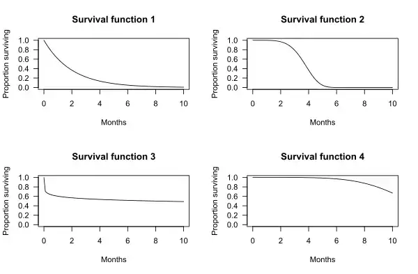
The graphs below show examples of hypothetical survival functions. The x-axis is time. The y-axis is the proportion of subjects surviving. The graphs show the probability that a subject will survive beyond time t.

Four survival functions

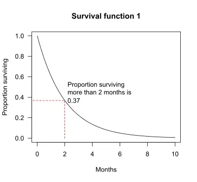
For example, for survival function 1, the probability of surviving longer than t = 2 months is 0.37. That is, 37% of subjects survive more than 2 months.

Survival function 1

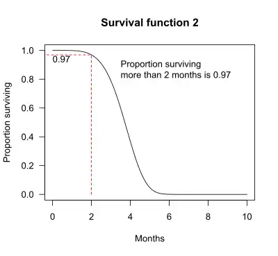
For survival function 2, the probability of surviving longer than t = 2 months is 0.97. That is, 97% of subjects survive more than 2 months.

Survival function 2

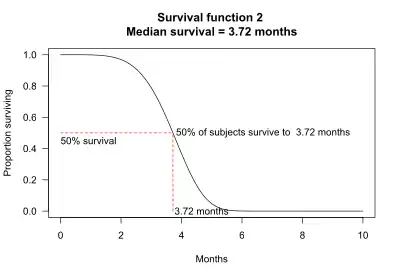
Median survival may be determined from the survival function: The median survival is the point where the survival function intersects the value 0.5.[4] For example, for survival function 2, 50% of the subjects survive 3.72 months. Median survival is thus 3.72 months.

Survival function with indicated median survival

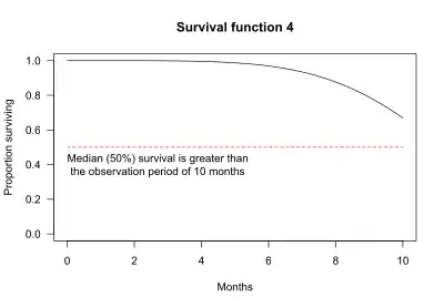
In some cases, median survival cannot be determined from the graph. For example, for survival function 4, more than 50% of the subjects survive longer than the observation period of 10 months.

Median survival greater than 10 months

The survival function is one of several ways to describe and display survival data. Another useful way to display data is a graph showing the distribution of survival times of subjects. Olkin,[5] page 426, gives the following example of survival data. The number of hours between successive failures of an air-conditioning system were recorded. The time between successive failures are 1, 3, 5, 7, 11, 11, 11, 12, 14, 14, 14, 16, 16, 20, 21, 23, 42, 47, 52, 62, 71, 71, 87, 90, 95, 120, 120, 225, 246, and 261 hours. The mean time between failures is 59.6. This mean value will be used shortly to fit a theoretical curve to the data. The figure below shows the distribution of the time between failures. The blue tick marks beneath the graph are the actual hours between successive failures.

Distribution of AC failure times

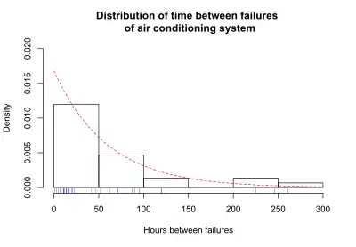
The distribution of failure times is over-laid with a curve representing an exponential distribution. For this example, the exponential distribution approximates the distribution of failure times. The exponential curve is a theoretical distribution fitted to the actual failure times. This particular exponential curve is specified by the parameter lambda, λ= 1/(mean time between failures) = 1/59.6 = 0.0168. The distribution of failure times is called the probability density function (pdf), if time can take any positive value. In equations, the pdf is specified as f(t). If time can only take discrete values (such as 1 day, 2 days, and so on), the distribution of failure times is called the probability mass function (pmf). Most survival analysis methods assume that time can take any positive value, and f(t) is the pdf. If the time between observed air conditioner failures is approximated using the exponential function, then the exponential curve gives the probability density function, f(t), for air conditioner failure times.

Another useful way to display the survival data is a graph showing the cumulative failures up to each time point. These data may be displayed as either the cumulative number or the cumulative proportion of failures up to each time. The graph below shows the cumulative probability (or proportion) of failures at each time for the air conditioning system. The stairstep line in black shows the cumulative proportion of failures. For each step there is a blue tick at the bottom of the graph indicating an observed failure time. The smooth red line represents the exponential curve fitted to the observed data.

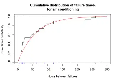
A graph of the cumulative probability of failures up to each time point is called the cumulative distribution function, or CDF. In survival analysis, the cumulative distribution function gives the probability that the survival time is less than or equal to a specific time, t.

Let T be survival time, which is any positive number. A particular time is designated by the lower case letter t. The cumulative distribution function of T is the function

${\displaystyle F(t)=\operatorname {P} (T\leq t),}$

where the right-hand side represents the probability that the random variable T is less than or equal to t. If time can take on any positive value, then the cumulative distribution function F(t) is the integral of the probability density function f(t).

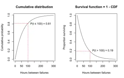
For the air conditioning example, the graph of the CDF below illustrates that the probability that the time to failure is less than or equal to 100 hours is 0.81, as estimated using the exponential curve fit to the data.

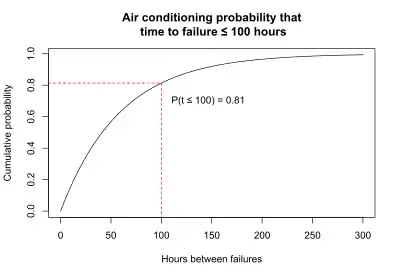
An alternative to graphing the probability that the failure time is less than or equal to 100 hours is to graph the probability that the failure time is greater than 100 hours. The probability that the failure time is greater than 100 hours must be 1 minus the probability that the failure time is less than or equal to 100 hours, because total probability must sum to 1.

This gives

P(failure time > 100 hours) = 1 - P(failure time < 100 hours) = 1 – 0.81 = 0.19.

This relationship generalizes to all failure times:

P(T > t) = 1 - P(T < t) = 1 – cumulative distribution function.

This relationship is shown on the graphs below. The graph on the left is the cumulative distribution function, which is P(T < t). The graph on the right is P(T > t) = 1 - P(T < t). The graph on the right is the survival function, S(t). The fact that the S(t) = 1 – CDF is the reason that another name for the survival function is the complementary cumulative distribution function.

In some cases, such as the air conditioner example, the distribution of survival times may be approximated well by a function such as the exponential distribution. Several distributions are commonly used in survival analysis, including the exponential, Weibull, gamma, normal, log-normal, and log-logistic.[3][6] These distributions are defined by parameters. The normal (Gaussian) distribution, for example, is defined by the two parameters mean and standard deviation. Survival functions that are defined by parameters are said to be parametric.

In the four survival function graphs shown above, the shape of the survival function is defined by a particular probability distribution: survival function 1 is defined by an exponential distribution, 2 is defined by a Weibull distribution, 3 is defined by a log-logistic distribution, and 4 is defined by another Weibull distribution.

A parametric model of survival may not be possible or desirable. In these situations, the most common method to model the survival function is the non-parametric Kaplan–Meier estimator. This estimator requires lifetime data. Periodic case (cohort) and death (and recovery) counts are statistically sufficient to make non-parametric maximum likelihood and least squares estimates of survival functions, without lifetime data.

• Every survival function ${\displaystyle S(t)}$ is monotonically decreasing, i.e. ${\displaystyle S(u)\leq S(t)}$ for all ${\displaystyle u>t}$.
  • It is a property of a random variable that maps a set of events, usually associated with mortality or failure of some system, onto time.
• The time, ${\displaystyle t=0}$, represents some origin, typically the beginning of a study or the start of operation of some system. ${\displaystyle S(0)}$ is commonly unity but can be less to represent the probability that the system fails immediately upon operation.
• Since the CDF is a right-continuous function, the survival function ${\displaystyle S(t)=1-F(t)}$ is also right-continuous.
• The survival function can be related to the probability density function ${\displaystyle f(t)}$ and the hazard function ${\displaystyle \lambda (t)}$
  • ${\displaystyle f(t)=-S'(t)}$
  • ${\displaystyle \lambda (t)=-{d \over {dt}}\log S(t)}$

So that ${\displaystyle S(t)=\exp[-\int _{0}^{t}\lambda (t')dt']}$

• The expected survival time ${\displaystyle \mathbb {E} (T)=\int _{0}^{\infty }S(t)dt}$

Proof of expected survival time formula

The expected value of a random variable ${\displaystyle T\in [0,\infty )}$ is defined as: ${\displaystyle \mathbb {E} (T)=\int _{0}^{\infty }tf(t)dt}$ where ${\displaystyle f(t)}$ is the probability density function. Using the relation ${\displaystyle f(t)=-S'(t)}$, the expected value formula may be modified: ${\displaystyle \mathbb {E} (T)=-\int _{0}^{\infty }tS'(t)dt}$ This may be further simplified by employing integration by parts: ${\displaystyle -\int _{0}^{\infty }tS'(t)dt=-tS(t){\bigg |}_{0}^{\infty }+\int _{0}^{\infty }S(t)dt}$ By definition, ${\displaystyle S(\infty )=0}$, meaning that the boundary terms are identically equal to zero. Therefore, we may conclude that the expected value is simply the integral of the survival function: ${\displaystyle \mathbb {E} (T)=\int _{0}^{\infty }S(t)dt}$

• Failure rate
• Frequency of exceedance
• Kaplan–Meier estimator
• Mean time to failure
• Residence time (statistics)
• Survivorship curve

References

- Kleinbaum, David G.; Klein, Mitchel (2012), Survival analysis: A Self-learning text (Third ed.), Springer, ISBN 978-1441966452
- Tableman, Mara; Kim, Jong Sung (2003), Survival Analysis Using S (First ed.), Chapman and Hall/CRC, ISBN 978-1584884088
- Ebeling, Charles (2010), An Introduction to Reliability and Maintainability Engineering (Second ed.), Waveland Press, ISBN 978-1577666257
- Machin, D., Cheung, Y. B., Parmar, M. (2006). Survival Analysis: A Practical Approach. Deutschland: Wiley. Page 36 and following Google Books
- Olkin, Ingram; Gleser, Leon; Derman, Cyrus (1994), Probability Models and Applications (Second ed.), Macmillan, ISBN 0-02-389220-X
- Klein, John; Moeschberger, Melvin (2005), Survival Analysis: Techniques for Censored and Truncated Data (Second ed.), Springer, ISBN 978-0387953991
- Mendenhall, William; Terry, Sincich (2007), Statistics for Engineering and the Sciences (Fifth ed.), Pearson / Prentice Hall, ISBN 978-0131877061
- Brostrom, Göran (2012), Event History Analysis with R (First ed.), Chapman & Hall/CRC, ISBN 978-1439831649
- Efron, Bradley; Hastie, Trevor (2016), Computer Age Statistical Inference: Algorithms, Evidence, and Data Science (First ed.), Cambridge University Press, ISBN 978-1107149892
- Lawless, Jerald (2002), Statistical Models and Methods for Lifetime Data (Second ed.), Wiley, ISBN 978-0471372158