Climate model
Numerical climate models use quantitative methods to simulate the interactions of the important drivers of climate, including atmosphere, oceans, land surface and ice. They are used for a variety of purposes from study of the dynamics of the climate system to projections of future climate. Climate models may also be qualitative (i.e. not numerical) models and also narratives, largely descriptive, of possible futures.[1]
Quantitative climate models take account of incoming energy from the sun as short wave electromagnetic radiation, chiefly visible and short-wave (near) infrared, as well as outgoing long wave (far) infrared electromagnetic. An imbalance results in a change in temperature.
Quantitative models vary in complexity. For example, a simple radiant heat transfer model treats the earth as a single point and averages outgoing energy. This can be expanded vertically (radiative-convective models) and/or horizontally. Coupled atmosphere–ocean–sea ice global climate models solve the full equations for mass and energy transfer and radiant exchange. In addition, other types of modelling can be interlinked, such as land use, in Earth System Models, allowing researchers to predict the interaction between climate and ecosystems.
Box models
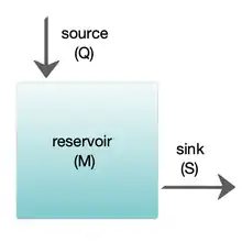
Box models are simplified versions of complex systems, reducing them to boxes (or reservoirs) linked by fluxes. The boxes are assumed to be mixed homogeneously. Within a given box, the concentration of any chemical species is therefore uniform. However, the abundance of a species within a given box may vary as a function of time due to the input to (or loss from) the box or due to the production, consumption or decay of this species within the box.
Simple box models, i.e. box model with a small number of boxes whose properties (e.g. their volume) do not change with time, are often useful to derive analytical formulas describing the dynamics and steady-state abundance of a species. More complex box models are usually solved using numerical techniques.
Box models are used extensively to model environmental systems or ecosystems and in studies of ocean circulation and the carbon cycle.[2] They are instances of a multi-compartment model.
Zero-dimensional models
Zero-dimensional models are also commonly referred to as Energy Balance Models (or EBM's).
Model with combined surface and atmosphere
A very simple model of the radiative equilibrium of the Earth is

where
- the left hand side represents the incoming energy from the Sun
- the right hand side represents the outgoing energy from the Earth, calculated from the Stefan–Boltzmann law assuming a model-fictive temperature, T, sometimes called the 'equilibrium temperature of the Earth', that is to be found,
and
- S is the solar constant – the incoming solar radiation per unit area—about 1367 W·m−2
- is the Earth's average albedo, measured to be 0.3.[3][4]
- r is Earth's radius—approximately 6.371×10⁶m
- π is the mathematical constant (3.141...)
- is the Stefan–Boltzmann constant—approximately 5.67×10⁻⁸ J·K−4·m−2·s−1
- is the effective emissivity of earth, about 0.612


The constant πr2 can be factored out, giving

Solving for the temperature,

This yields an apparent effective average Earth temperature of 288 K (15 °C; 59 °F).[5] This is because the above equation represents the effective radiative temperature of Earth's combined surface and atmosphere (including clouds).
This very simple model is quite instructive. For example, it easily determines the change in the effective temperature caused by changes in solar constant, Earth albedo, or effective Earth emissivity.
The average emissivity of the earth is readily estimated from available data. The emissivities of terrestrial surfaces are all in the range of 0.96 to 0.99[6][7] (except for some small desert areas which may be as low as 0.7). Clouds, however, which cover about half of the earth's surface, have an average emissivity of about 0.5[8] (which must be reduced by the fourth power of the ratio of cloud absolute temperature to average earth absolute temperature) and an average cloud temperature of about 258 K (−15 °C; 5 °F).[9] Taking all this properly into account results in an effective earth emissivity of about 0.64 (earth average temperature 285 K (12 °C; 53 °F)).
Models with separated surface and atmospheric layers
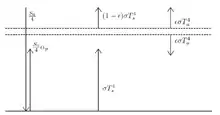
Dimensionless models have also been constructed with functionally separated atmospheric layers from the surface. The simplest of these is the zero-dimensional, one-layer model,[10] which may be readily extended to an arbitrary number of atmospheric layers.[11] The surface and atmospheric layer(s) are each characterized by a corresponding temperature and emissivity value, but no thickness. Applying radiative equilibrium (i.e conservation of energy) at the interfaces between layers produces a set of coupled equations which are solvable.
Layered models produce temperatures that better estimate those observed for Earth's surface and atmospheric levels.[12] They likewise illustrate the radiative heat transfer processes which underlie the greenhouse effect. Quantification of this phenomenon using a version of the one-layer model was first published by Svante Arrhenius in year 1896.[13]
Radiative-convective models
The zero-dimensional model above, using the solar constant and given average earth temperature, determines the effective earth emissivity of long wave radiation emitted to space. This can be refined in the vertical to a one-dimensional radiative-convective model, which considers two processes of energy transport:
- upwelling and downwelling radiative transfer through atmospheric layers that both absorb and emit infrared radiation
- upward transport of heat by convection (especially important in the lower troposphere).
The radiative-convective models have advantages over the simple model: they can determine the effects of varying greenhouse gas concentrations on effective emissivity and therefore the surface temperature. But added parameters are needed to determine local emissivity and albedo and address the factors that move energy about the earth.
Effect of ice-albedo feedback on global sensitivity in a one-dimensional radiative-convective climate model.[14][15][16]
Higher-dimension models
The zero-dimensional model may be expanded to consider the energy transported horizontally in the atmosphere. This kind of model may well be zonally averaged. This model has the advantage of allowing a rational dependence of local albedo and emissivity on temperature – the poles can be allowed to be icy and the equator warm – but the lack of true dynamics means that horizontal transports have to be specified.[17]
EMICs (Earth-system models of intermediate complexity)
Depending on the nature of questions asked and the pertinent time scales, there are, on the one extreme, conceptual, more inductive models, and, on the other extreme, general circulation models operating at the highest spatial and temporal resolution currently feasible. Models of intermediate complexity bridge the gap. One example is the Climber-3 model. Its atmosphere is a 2.5-dimensional statistical-dynamical model with 7.5° × 22.5° resolution and time step of half a day; the ocean is MOM-3 (Modular Ocean Model) with a 3.75° × 3.75° grid and 24 vertical levels.[18]
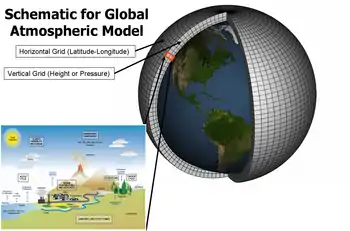
GCMs (global climate models or general circulation models)
General Circulation Models (GCMs) discretise the equations for fluid motion and energy transfer and integrate these over time. Unlike simpler models, GCMs divide the atmosphere and/or oceans into grids of discrete "cells", which represent computational units. Unlike simpler models which make mixing assumptions, processes internal to a cell—such as convection—that occur on scales too small to be resolved directly are parameterised at the cell level, while other functions govern the interface between cells.
Atmospheric GCMs (AGCMs) model the atmosphere and impose sea surface temperatures as boundary conditions. Coupled atmosphere-ocean GCMs (AOGCMs, e.g. HadCM3, EdGCM, GFDL CM2.X, ARPEGE-Climat)[19] combine the two models. The first general circulation climate model that combined both oceanic and atmospheric processes was developed in the late 1960s at the NOAA Geophysical Fluid Dynamics Laboratory[20] AOGCMs represent the pinnacle of complexity in climate models and internalise as many processes as possible. However, they are still under development and uncertainties remain. They may be coupled to models of other processes, such as the carbon cycle, so as to better model feedback effects. Such integrated multi-system models are sometimes referred to as either "earth system models" or "global climate models."
Research and development
There are three major types of institution where climate models are developed, implemented and used:
- National meteorological services. Most national weather services have a climatology section.
- Universities. Relevant departments include atmospheric sciences, meteorology, climatology, and geography.
- National and international research laboratories. Examples include the National Center for Atmospheric Research (NCAR, in Boulder, Colorado, USA), the Geophysical Fluid Dynamics Laboratory (GFDL, in Princeton, New Jersey, USA), Los Alamos National Laboratory, the Hadley Centre for Climate Prediction and Research (in Exeter, UK), the Max Planck Institute for Meteorology in Hamburg, Germany, or the Laboratoire des Sciences du Climat et de l'Environnement (LSCE), France, to name but a few.
The World Climate Research Programme (WCRP), hosted by the World Meteorological Organization (WMO), coordinates research activities on climate modelling worldwide.
A 2012 U.S. National Research Council report discussed how the large and diverse U.S. climate modeling enterprise could evolve to become more unified.[21] Efficiencies could be gained by developing a common software infrastructure shared by all U.S. climate researchers, and holding an annual climate modeling forum, the report found.[22]
See also
- Atmospheric reanalysis
- General circulation model
- Chemical transport model
- Atmospheric Radiation Measurement (ARM) (in the US)
- Climate Data Exchange
- Climateprediction.net
- GFDL CM2.X
- GO-ESSP
- Numerical Weather Prediction
- Static atmospheric model
- Tropical cyclone prediction model
- Verification and validation of computer simulation models
- CICE sea ice model
Climate models on the web
- Dapper/DChart — plot and download model data referenced by the Fourth Assessment Report (AR4) of the Intergovernmental Panel on Climate Change. (No longer available)
- NCAR/UCAR Community Climate System Model (CCSM)
- Do it yourself climate prediction
- Primary research GCM developed by NASA/GISS (Goddard Institute for Space Studies)
- Original NASA/GISS global climate model (GCM) with a user-friendly interface for PCs and Macs
- CCCma model info and interface to retrieve model data
- NOAA/Geophysical Fluid Dynamics Laboratory CM2 global climate model info and model output data files
- Dry idealized AGCM based on above GFDL CM2[23]
- Model of an idealized Moist Atmosphere (MiMA): based on GFDL CM2. Complexity in-between dry models and full GCMs[24]
- University of Victoria Global climate model, free for download. Leading researcher was a contributing author to an IPCC report on climate change.
- vimeo.com/user12523377/videos Visualizations of climate models of ETH Zurich
- Empirical Climate Model Archived 24 March 2019 at the Wayback Machine
References
- IPCC (2014). "AR5 Synthesis Report - Climate Change 2014. Contribution of Working Groups I, II and III to the Fifth Assessment Report of the Intergovernmental Panel on Climate Change" (PDF): 58.
Box 2.3. ‘Models’ are typically numerical simulations of real-world systems, calibrated and validated using observations from experiments or analogies, and then run using input data representing future climate. Models can also include largely descriptive narratives of possible futures, such as those used in scenario construction. Quantitative and descriptive models are often used together.
{{cite journal}}: Cite journal requires|journal=(help) - Sarmiento, J.L.; Toggweiler, J.R. (1984). "A new model for the role of the oceans in determining atmospheric P CO 2". Nature. 308 (5960): 621–24. Bibcode:1984Natur.308..621S. doi:10.1038/308621a0. S2CID 4312683.
- Goode, P. R.; et al. (2001). "Earthshine Observations of the Earth's Reflectance" (PDF). Geophys. Res. Lett. 28 (9): 1671–4. Bibcode:2001GeoRL..28.1671G. doi:10.1029/2000GL012580. S2CID 34790317.
- "Scientists Watch Dark Side of the Moon to Monitor Earth's Climate". American Geophysical Union. 17 April 2001.
- Archived 18 February 2013 at the Wayback Machine
- "Seawater Samples - Emissivities". ucsb.edu.
- Jin M, Liang S (15 June 2006). "An Improved Land Surface Emissivity Parameter for Land Surface Models Using Global Remote Sensing Observations" (PDF). J. Climate. 19 (12): 2867–81. Bibcode:2006JCli...19.2867J. doi:10.1175/JCLI3720.1.
- T.R. Shippert; S.A. Clough; P.D. Brown; W.L. Smith; R.O. Knuteson; S.A. Ackerman. "Spectral Cloud Emissivities from LBLRTM/AERI QME" (PDF). Proceedings of the Eighth Atmospheric Radiation Measurement (ARM) Science Team Meeting March 1998 Tucson, Arizona.
- A.G. Gorelik; V. Sterljadkin; E. Kadygrov; A. Koldaev. "Microwave and IR Radiometry for Estimation of Atmospheric Radiation Balance and Sea Ice Formation" (PDF). Proceedings of the Eleventh Atmospheric Radiation Measurement (ARM) Science Team Meeting March 2001 Atlanta, Georgia.
- "ACS Climate Science Toolkit - Atmospheric Warming - A Single-Layer Atmosphere Model". American Chemical Society. Retrieved 2 October 2022.
- "ACS Climate Science Toolkit - Atmospheric Warming - A Multi-Layer Atmosphere Model". American Chemical Society. Retrieved 2 October 2022.
- "METEO 469: From Meteorology to Mitigation - Understanding Global Warming - Lesson 5 - Modelling of the Climate System - One-Layer Energy Balance Model". Penn State College of Mineral and Earth Sciences - Department of Meteorology and Atmospheric Sciences. Retrieved 2 October 2022.
- Svante Arrhenius (1896). "On the influence of carbonic acid in the air upon the temperature of the ground". Philosophical Magazine and Journal of Science. 41 (251): 237–276. doi:10.1080/14786449608620846.
- "Pubs.GISS: Wang and Stone 1980: Effect of ice-albedo feedback on global sensitivity in a one-dimensional..." nasa.gov. Archived from the original on 30 July 2012.
- Wang, W.C.; P.H. Stone (1980). "Effect of ice-albedo feedback on global sensitivity in a one-dimensional radiative-convective climate model". J. Atmos. Sci. 37 (3): 545–52. Bibcode:1980JAtS...37..545W. doi:10.1175/1520-0469(1980)037<0545:EOIAFO>2.0.CO;2.
- "Climate Change 2001: The Scientific Basis". grida.no. Archived from the original on 25 March 2003.
- "Energy Balance Models". shodor.org.
- "emics1". pik-potsdam.de.
- Archived 27 September 2007 at the Wayback Machine
- "NOAA 200th Top Tens: Breakthroughs: The First Climate Model". noaa.gov.
- "U.S. National Research Council Report, A National Strategy for Advancing Climate Modeling". Archived from the original on 3 October 2012. Retrieved 18 January 2021.
- "U.S. National Research Council Report-in-Brief, A National Strategy for Advancing Climate Modeling". Archived from the original on 18 October 2012. Retrieved 3 October 2012.
- M. Jucker, S. Fueglistaler and G. K. Vallis "Stratospheric sudden warmings in an idealized GCM". Journal of Geophysical Research: Atmospheres 2014 119 (19) 11,054-11,064; doi:10.1002/2014JD022170
- M. Jucker and E. P. Gerber: "Untangling the Annual Cycle of the Tropical Tropopause Layer with an Idealized Moist Model". Journal of Climate 2017 30 (18) 7339-7358; doi:10.1175/JCLI-D-17-0127.1
Bibliography
- Roulstone, Ian; Norbury, John (2013). Invisible in the Storm: the role of mathematics in understanding weather. Princeton University Press.
External links
- Coupled Model Intercomparison Project
- On the Radiative and Dynamical Feedbacks over the Equatorial Pacific Cold Tongue
- Basic Radiation Calculations — The Discovery of Global Warming
- Henderson-Sellers, A.; Robinson, P. J. (1999). Contemporary Climatology. New York: Longman. ISBN 978-0-582-27631-4. Archived from the original on 28 September 2007.
- Climate Modeling 101 website by the U.S. National Research Council — This site is a primer on how climate models work. The information is based on expert, consensus reports from the U.S. National Research Council's Board on Atmospheric Sciences and Climate. The most recent is A National Strategy for Advancing Climate Modeling Archived 3 October 2012 at the Wayback Machine.
- Why results from the next generation of climate models matter CarbonBrief, Guest post by Belcher, Boucher, Sutton, 21 March 2019
- Builder Insight - Modelling the Future Climate in Passively Cooled Buildings
| |||||||||||||
| |||||||||||||
| |||||||||||||
| |||||||||||||
| |||||||||||||
| |||||||||||||
| |||||||||||||
| |||||||||||||