Estimator

For a given sample ${\displaystyle x}$, the "error" of the estimator ${\displaystyle {\widehat {\theta }}}$ is defined as

${\displaystyle e(x)={\widehat {\theta }}(x)-\theta ,}$

where ${\displaystyle \theta }$ is the parameter being estimated. The error, e, depends not only on the estimator (the estimation formula or procedure), but also on the sample.

The mean squared error of ${\displaystyle {\widehat {\theta }}}$ is defined as the expected value (probability-weighted average, over all samples) of the squared errors; that is,

${\displaystyle \operatorname {MSE} ({\widehat {\theta }})=\operatorname {E} [({\widehat {\theta }}(X)-\theta )^{2}].}$

It is used to indicate how far, on average, the collection of estimates are from the single parameter being estimated. Consider the following analogy. Suppose the parameter is the bull's-eye of a target, the estimator is the process of shooting arrows at the target, and the individual arrows are estimates (samples). Then high MSE means the average distance of the arrows from the bull's eye is high, and low MSE means the average distance from the bull's eye is low. The arrows may or may not be clustered. For example, even if all arrows hit the same point, yet grossly miss the target, the MSE is still relatively large. However, if the MSE is relatively low then the arrows are likely more highly clustered (than highly dispersed) around the target.

For a given sample ${\displaystyle x}$, the sampling deviation of the estimator ${\displaystyle {\widehat {\theta }}}$ is defined as

${\displaystyle d(x)={\widehat {\theta }}(x)-\operatorname {E} ({\widehat {\theta }}(X))={\widehat {\theta }}(x)-\operatorname {E} ({\widehat {\theta }}),}$

where ${\displaystyle \operatorname {E} ({\widehat {\theta }}(X))}$ is the expected value of the estimator. The sampling deviation, d, depends not only on the estimator, but also on the sample.

The variance of ${\displaystyle {\widehat {\theta }}}$ is the expected value of the squared sampling deviations; that is, ${\displaystyle \operatorname {Var} ({\widehat {\theta }})=\operatorname {E} [({\widehat {\theta }}-\operatorname {E} [{\widehat {\theta }}])^{2}]}$. It is used to indicate how far, on average, the collection of estimates are from the expected value of the estimates. (Note the difference between MSE and variance.) If the parameter is the bull's-eye of a target, and the arrows are estimates, then a relatively high variance means the arrows are dispersed, and a relatively low variance means the arrows are clustered. Even if the variance is low, the cluster of arrows may still be far off-target, and even if the variance is high, the diffuse collection of arrows may still be unbiased. Finally, even if all arrows grossly miss the target, if they nevertheless all hit the same point, the variance is zero.

The bias of ${\displaystyle {\widehat {\theta }}}$ is defined as ${\displaystyle B({\widehat {\theta }})=\operatorname {E} ({\widehat {\theta }})-\theta }$. It is the distance between the average of the collection of estimates, and the single parameter being estimated. The bias of ${\displaystyle {\widehat {\theta }}}$ is a function of the true value of ${\displaystyle \theta }$ so saying that the bias of ${\displaystyle {\widehat {\theta }}}$ is ${\displaystyle b}$ means that for every ${\displaystyle \theta }$ the bias of ${\displaystyle {\widehat {\theta }}}$ is ${\displaystyle b}$.

There are two kinds of estimators: biased estimators and unbiased estimators. Whether an estimator is biased or not can be identified by the relationship between ${\displaystyle \operatorname {E} ({\widehat {\theta }})-\theta }$ and 0:

• If ${\displaystyle \operatorname {E} ({\widehat {\theta }})-\theta \neq 0}$, ${\displaystyle {\widehat {\theta }}}$ is biased.
• If ${\displaystyle \operatorname {E} ({\widehat {\theta }})-\theta =0}$, ${\displaystyle {\widehat {\theta }}}$ is unbiased.

The bias is also the expected value of the error, since ${\displaystyle \operatorname {E} ({\widehat {\theta }})-\theta =\operatorname {E} ({\widehat {\theta }}-\theta )}$. If the parameter is the bull's eye of a target and the arrows are estimates, then a relatively high absolute value for the bias means the average position of the arrows is off-target, and a relatively low absolute bias means the average position of the arrows is on target. They may be dispersed, or may be clustered. The relationship between bias and variance is analogous to the relationship between accuracy and precision.

The estimator ${\displaystyle {\widehat {\theta }}}$ is an unbiased estimator of ${\displaystyle \theta }$ if and only if ${\displaystyle B({\widehat {\theta }})=0}$. Bias is a property of the estimator, not of the estimate. Often, people refer to a "biased estimate" or an "unbiased estimate," but they really are talking about an "estimate from a biased estimator," or an "estimate from an unbiased estimator." Also, people often confuse the "error" of a single estimate with the "bias" of an estimator. That the error for one estimate is large, does not mean the estimator is biased. In fact, even if all estimates have astronomical absolute values for their errors, if the expected value of the error is zero, the estimator is unbiased. Also, an estimator's being biased does not preclude the error of an estimate from being zero in a particular instance. The ideal situation is to have an unbiased estimator with low variance, and also try to limit the number of samples where the error is extreme (that is, have few outliers). Yet unbiasedness is not essential. Often, if just a little bias is permitted, then an estimator can be found with lower mean squared error and/or fewer outlier sample estimates.

An alternative to the version of "unbiased" above, is "median-unbiased", where the median of the distribution of estimates agrees with the true value; thus, in the long run half the estimates will be too low and half too high. While this applies immediately only to scalar-valued estimators, it can be extended to any measure of central tendency of a distribution: see median-unbiased estimators.

In a practical problem, ${\displaystyle {\widehat {\theta }}}$ can always have functional relationship with ${\displaystyle \theta }$. For example, A genetic theory states there is a type of leave, starchy green, occur with probability ${\displaystyle p_{1}=1/4\cdot (\theta +2)}$, with ${\displaystyle 0<\theta <1}$. For ${\displaystyle n}$ leaves, the random variable ${\displaystyle N_{1}}$, the number of starchy green leaves, can be modeled with a ${\displaystyle Bin(n,p_{1})}$ distribution. The number can be used to express the following estimator for ${\displaystyle \theta }$: ${\displaystyle {\widehat {\theta }}=4/n\cdot N_{1}-2}$. One can show that ${\displaystyle {\widehat {\theta }}}$ is an unbiased estimator for ${\displaystyle \theta }$: ${\displaystyle E[{\widehat {\theta }}]=E[4/n\cdot N_{1}-2]}$ ${\displaystyle =4/n\cdot E[N_{1}]-2}$ ${\displaystyle =4/n\cdot np_{1}-2}$ ${\displaystyle =4\cdot p_{1}-2}$ ${\displaystyle =4\cdot 1/4\cdot (\theta +2)-2}$ ${\displaystyle =\theta +2-2}$ ${\displaystyle =\theta }$.

• The mean squared error, variance, and bias, are related: ${\displaystyle \operatorname {MSE} ({\widehat {\theta }})=\operatorname {Var} ({\widehat {\theta }})+(B({\widehat {\theta }}))^{2},}$ i.e. mean squared error = variance + square of bias. In particular, for an unbiased estimator, the variance equals the mean squared error.
• The standard deviation of an estimator ${\displaystyle {\widehat {\theta }}}$ of ${\displaystyle \theta }$ (the square root of the variance), or an estimate of the standard deviation of an estimator ${\displaystyle {\widehat {\theta }}}$ of ${\displaystyle \theta }$, is called the standard error of ${\displaystyle {\widehat {\theta }}}$.
• The bias-variance tradeoff will be used in model complexity, over-fitting and under-fitting. It is mainly used in the field of supervised learning and predictive modeling to diagnose the performance of algorithms.

A consistent sequence of estimators is a sequence of estimators that converge in probability to the quantity being estimated as the index (usually the sample size) grows without bound. In other words, increasing the sample size increases the probability of the estimator being close to the population parameter.

Mathematically, a sequence of estimators {t_n; n ≥ 0} is a consistent estimator for parameter θ if and only if, for all ε > 0, no matter how small, we have

${\displaystyle \lim _{n\to \infty }\Pr \left\{\left|t_{n}-\theta \right|<\varepsilon \right\}=1}$.

The consistency defined above may be called weak consistency. The sequence is strongly consistent, if it converges almost surely to the true value.

An estimator that converges to a multiple of a parameter can be made into a consistent estimator by multiplying the estimator by a scale factor, namely the true value divided by the asymptotic value of the estimator. This occurs frequently in estimation of scale parameters by measures of statistical dispersion.

An asymptotically normal estimator is a consistent estimator whose distribution around the true parameter θ approaches a normal distribution with standard deviation shrinking in proportion to ${\displaystyle 1/{\sqrt {n}}}$ as the sample size n grows. Using ${\displaystyle {\xrightarrow {D}}}$ to denote convergence in distribution, t_n is asymptotically normal if

${\displaystyle {\sqrt {n}}(t_{n}-\theta ){\xrightarrow {D}}N(0,V),}$

for some V.

In this formulation V/n can be called the asymptotic variance of the estimator. However, some authors also call V the asymptotic variance. Note that convergence will not necessarily have occurred for any finite "n", therefore this value is only an approximation to the true variance of the estimator, while in the limit the asymptotic variance (V/n) is simply zero. To be more specific, the distribution of the estimator t_n converges weakly to a dirac delta function centered at ${\displaystyle \theta }$.

The central limit theorem implies asymptotic normality of the sample mean ${\displaystyle {\bar {X}}}$ as an estimator of the true mean. More generally, maximum likelihood estimators are asymptotically normal under fairly weak regularity conditions — see the asymptotics section of the maximum likelihood article. However, not all estimators are asymptotically normal; the simplest examples are found when the true value of a parameter lies on the boundary of the allowable parameter region.

The efficiency of an estimator is used to estimate the quantity of interest in a "minimum error" manner. In reality, there is not an explicit best estimator; there can only be a better estimator. The good or not of the efficiency of an estimator is based on the choice of a particular loss function, and it is reflected by two naturally desirable properties of estimators: to be unbiased ${\displaystyle \operatorname {E} ({\widehat {\theta }})-\theta =0}$ and have minimal mean squared error (MSE) ${\displaystyle \operatorname {E} [({\widehat {\theta }}-\theta )^{2}]}$. These cannot in general both be satisfied simultaneously: an unbiased estimator may have a lower mean squared error than any biased estimator (see estimator bias). A function relates the mean squared error with the estimator bias.[4]

${\displaystyle \operatorname {E} [({\widehat {\theta }}-\theta )^{2}]=(\operatorname {E} ({\widehat {\theta }})-\theta )^{2}+\operatorname {Var} (\theta )\ }$

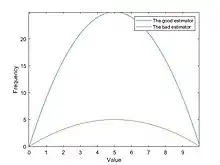
The first term represents the mean squared error; the second term represents the square of the estimator bias; and the third term represents the variance of the sample. The quality of the estimator can be identified from the comparison between the variance, the square of the estimator bias, or the MSE. The variance of the good estimator (good efficiency) would be smaller than the variance of the bad estimator (bad efficiency). The square of a estimator bias with a good estimator would be smaller than the estimator bias with a bad estimator. The MSE of a good estimator would be smaller than the MSE of the bad estimator. Suppose there are two estimator, ${\displaystyle \theta _{1}}$ is the good estimator and ${\displaystyle \theta _{2}}$ is the bad estimator. The above relationship can be expressed by the following formulas.

${\displaystyle \operatorname {Var} (\theta _{1})<\operatorname {Var} (\theta _{2})}$

${\displaystyle |\operatorname {E} ({\theta }_{1})-\theta |<|\operatorname {E} ({\theta _{2}})-\theta |}$

${\displaystyle \operatorname {MSE} (\theta _{1})<\operatorname {MSE} (\theta _{2})}$

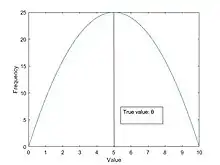
Besides using formula to identify the efficiency of the estimator, it can also be identified through the graph. If an estimator is efficient, in the frequency vs. value graph, there will be a curve with high frequency at the center and low frequency on the two sides. For example:

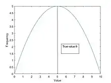
If an estimator is not efficient, the frequency vs. value graph, there will be a relatively more gentle curve.

To put it simply, the good estimator has a narrow curve, while the bad estimator has a large curve. Plotting these two curves on one graph with a shared y-axis, the difference becomes more obvious.

Among unbiased estimators, there often exists one with the lowest variance, called the minimum variance unbiased estimator (MVUE). In some cases an unbiased efficient estimator exists, which, in addition to having the lowest variance among unbiased estimators, satisfies the Cramér–Rao bound, which is an absolute lower bound on variance for statistics of a variable.

Concerning such "best unbiased estimators", see also Cramér–Rao bound, Gauss–Markov theorem, Lehmann–Scheffé theorem, Rao–Blackwell theorem.

References

- Mosteller, F.; Tukey, J. W. (1987) [1968]. "Data Analysis, including Statistics". The Collected Works of John W. Tukey: Philosophy and Principles of Data Analysis 1965–1986. Vol. 4. CRC Press. pp. 601–720 [p. 633]. ISBN 0-534-05101-4 – via Google Books.
- Kosorok (2008), Section 3.1, pp 35–39.
- Jaynes (2007), p.172.
- Dekking, Frederik Michel; Kraaikamp, Cornelis; Lopuhaä, Hendrik Paul; Meester, Ludolf Erwin (2005). "A Modern Introduction to Probability and Statistics". Springer Texts in Statistics. doi:10.1007/1-84628-168-7. ISSN 1431-875X.
Further reading
- Bol'shev, Login Nikolaevich (2001) [1994], "Statistical estimator", Encyclopedia of Mathematics, EMS Press.
- Jaynes, E. T. (2007). Probability Theory: The logic of science (5 ed.). Cambridge University Press. ISBN 978-0-521-59271-0..
- Kosorok, Michael (2008). Introduction to Empirical Processes and Semiparametric Inference. Springer Series in Statistics. Springer. doi:10.1007/978-0-387-74978-5. ISBN 978-0-387-74978-5.
- Lehmann, E. L.; Casella, G. (1998). Theory of Point Estimation (2nd ed.). Springer. ISBN 0-387-98502-6.
- Shao, Jun (1998), Mathematical Statistics, Springer, ISBN 0-387-98674-X