Taxicab geometry
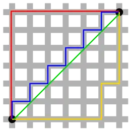
A taxicab geometry or a Manhattan geometry is a geometry in which the usual distance function or metric of Euclidean geometry is replaced by a new metric in which the distance between two points is the sum of the absolute differences of their Cartesian coordinates. The taxicab metric is also known as rectilinear distance, L1 distance, L1 distance or norm (see Lp space), snake distance, city block distance, Manhattan distance or Manhattan length, with corresponding variations in the name of the geometry.[1] The latter names allude to the grid layout of most streets on the island of Manhattan, which causes the shortest path a car could take between two intersections in the borough to have length equal to the intersections' distance in taxicab geometry.


The geometry has been used in regression analysis since the 18th century, and today is often referred to as LASSO. The geometric interpretation dates to non-Euclidean geometry of the 19th century and is due to Hermann Minkowski.
In two dimensions, the taxicab distance between two points and is . That is, it is the sum of the absolute values of the differences between both sets of coordinates.


Formal definition
The taxicab distance, , between two vectors in an n-dimensional real vector space with fixed Cartesian coordinate system, is the sum of the lengths of the projections of the line segment between the points onto the coordinate axes. More formally,


where are vectors


For example, in the plane, the taxicab distance between and is


Properties
Taxicab distance depends on the rotation of the coordinate system, but does not depend on its reflection about a coordinate axis or its translation. Taxicab geometry satisfies all of Hilbert's axioms (a formalization of Euclidean geometry) except for the side-angle-side axiom, as two triangles with equally "long" two sides and an identical angle between them are typically not congruent unless the mentioned sides happen to be parallel.
Balls
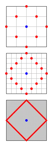
A topological ball is a set of points with a fixed distance, called the radius, from a point called the center. In n-dimensional Euclidean geometry, the balls are spheres. In taxicab geometry, distance is determined by a different metric than in Euclidean geometry, and the shape of the ball changes as well. In n dimensions, a taxicab ball is in the shape of an n-dimensional orthoplex. In two dimensions, these are squares with sides oriented at a 45° angle to the coordinate axes. The image to the right shows why this is true, by showing in red the set of all points with a fixed distance from a center, shown in blue. As the size of the city blocks diminishes, the points become more numerous and become a rotated square in a continuous taxicab geometry. While each side would have length using a Euclidean metric, where r is the circle's radius, its length in taxicab geometry is 2r. Thus, a circle's circumference is 8r. Thus, the value of a geometric analog to is 4 in this geometry. The formula for the unit circle in taxicab geometry is in Cartesian coordinates and


A circle of radius 1 (using this distance) is the von Neumann neighborhood of its center.
A circle of radius r for the Chebyshev distance (L∞ metric) on a plane is also a square with side length 2r parallel to the coordinate axes, so planar Chebyshev distance can be viewed as equivalent by rotation and scaling to planar taxicab distance. However, this equivalence between L1 and L∞ metrics does not generalize to higher dimensions.
Whenever each pair in a collection of these circles has a nonempty intersection, there exists an intersection point for the whole collection; therefore, the Manhattan distance forms an injective metric space.
Arc Length
Let be a continuously differentiable function in . Let be the taxicab arc length of the planar curve defined by on some interval . Then the taxicab length of the infinitesimal regular partition of the arc, , is given by:[2]


By the Mean Value Theorem, there exists some point between and such that .[3]


Then is given as the sum of every partition of on as they get arbitrarily small.

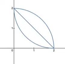
To test this, take the taxicab circle of radius centered at the origin. Its curve in the first quadrant is given by whose length is


Multiplying this value by to account for the remaining quadrants gives , which agrees with the circumference of a taxicab circle.[4] Now take the Euclidean circle of radius centered at the origin, which is given by . Its arc length in the first quadrant is given by


Accounting for the remaining quadrants gives again. Therefore, the circumference of the taxicab circle and the Euclidean circle in the taxicab metric are equal.[5] In fact, for any function that is monotonic and differentiable with a continuous derivative over an interval , the arc length of over is .[6]


Compressed sensing
In solving an underdetermined system of linear equations, the regularization term for the parameter vector is expressed in terms of the -norm (taxicab geometry) of the vector.[7] This approach appears in the signal recovery framework called compressed sensing.
Differences of frequency distributions
Taxicab geometry can be used to assess the differences in discrete frequency distributions. For example, in RNA splicing positional distributions of hexamers, which plot the probability of each hexamer appearing at each given nucleotide near a splice site, can be compared with L1-distance. Each position distribution can be represented as a vector where each entry represents the likelihood of the hexamer starting at a certain nucleotide. A large L1-distance between the two vectors indicates a significant difference in the nature of the distributions while a small distance denotes similarly shaped distributions. This is equivalent to measuring the area between the two distribution curves because the area of each segment is the absolute difference between the two curves' likelihoods at that point. When summed together for all segments, it provides the same measure as L1-distance.[8]
History
The L1 metric was used in regression analysis in 1757 by Roger Joseph Boscovich.[9] The geometric interpretation dates to the late 19th century and the development of non-Euclidean geometries, notably by Hermann Minkowski and his Minkowski inequality, of which this geometry is a special case, particularly used in the geometry of numbers, (Minkowski 1910). The formalization of Lp spaces is credited to (Riesz 1910).
See also
- Fifteen puzzle
- Hamming distance – Number of bits that differ between two strings
- Manhattan wiring
- Mannheim distance
- Metric
- Minkowski distance
- Normed vector space – Vector space on which a distance is defined
- Orthogonal convex hull – Minimal superset that intersects each axis-parallel line in an interval
- Random walk – Mathematical formalization of a path that consists of a succession of random steps
Notes
- Black, Paul E. "Manhattan distance". Dictionary of Algorithms and Data Structures. Retrieved October 6, 2019.
- Heinbockel, J.H. (2012). Introduction to Calculus Volume II. Old Dominion University. pp. 54–55.
- Penot, J.P. (1988-01-01). "On the mean value theorem". Optimization. 19 (2): 147–156. doi:10.1080/02331938808843330. ISSN 0233-1934.
- Petrovic, Maja; Malesevic, Branko; Banjac, Bojan; Obradovic, Ratko (2014-05-25). "Geometry of some taxicab curves". arXiv:1405.7579 [math]. doi:10.48550/arxiv.1405.7579.
- Kemp, Aubrey (2018-08-07). "Generalizing and Transferring Mathematical Definitions from Euclidean to Taxicab Geometry". Mathematics Dissertations. doi:10.57709/12521263.
- Thompson, Kevin P. (2011-01-14). "The Nature of Length, Area, and Volume in Taxicab Geometry". arXiv:1101.2922 [math]. doi:10.48550/arxiv.1101.2922.
- Donoho, David L. (March 23, 2006). "For most large underdetermined systems of linear equations the minimal -norm solution is also the sparsest solution". Communications on Pure and Applied Mathematics. 59 (6): 797–829. doi:10.1002/cpa.20132.
- Lim, Kian Huat; Ferraris, Luciana; Filloux, Madeleine E.; Raphael, Benjamin J.; Fairbrother, William G. (July 5, 2011). "Using positional distribution to identify splicing elements and predict pre-mRNA processing defects in human genes". Proceedings of the National Academy of Sciences of the United States of America. 108 (27): 11093–11098. Bibcode:2011PNAS..10811093H. doi:10.1073/pnas.1101135108. PMC 3131313. PMID 21685335.
- Stigler, Stephen M. (1986). The History of Statistics: The Measurement of Uncertainty before 1900. Harvard University Press. ISBN 9780674403406. Retrieved October 6, 2019.
References
- Krause, Eugene F. (1987). Taxicab Geometry. Dover. ISBN 978-0-486-25202-5.
- Minkowski, Hermann (1910). Geometrie der Zahlen (in German). Leipzig and Berlin: R. G. Teubner. JFM 41.0239.03. MR 0249269. Retrieved October 6, 2019.
- Riesz, Frigyes (1910). "Untersuchungen über Systeme integrierbarer Funktionen". Mathematische Annalen (in German). 69 (4): 449–497. doi:10.1007/BF01457637. hdl:10338.dmlcz/128558. S2CID 120242933.
External links
- Weisstein, Eric W. "Taxicab Metric". MathWorld.
- Malkevitch, Joe (October 1, 2007). "Taxi!". American Mathematical Society. Retrieved October 6, 2019.