The Poisson Random Variable

The Poisson Distribution and Its History

The Poisson distribution is a discrete probability distribution. It expresses the probability of a given number of events occurring in a fixed interval of time and/or space, if these events occur with a known average rate and independently of the time since the last event. The Poisson distribution can also be used for the number of events in other specified intervals such as distance, area, or volume.

For example: Let's suppose that, on average, a person typically receives four pieces of mail per day. There will be a certain spread—sometimes a little more, sometimes a little less, once in a while nothing at all. Given only the average rate for a certain period of observation (i.e., pieces of mail per day, phonecalls per hour, etc.), and assuming that the process that produces the event flow is essentially random, the Poisson distribution specifies how likely it is that the count will be 3, 5, 10, or any other number during one period of observation. It predicts the degree of spread around a known average rate of occurrence.

The distribution was first introduced by Siméon Denis Poisson (1781–1840) and published, together with his probability theory, in 1837 in his work Recherches sur la Probabilité des Jugements en Matière Criminelle et en Matière Civile ("Research on the Probability of Judgments in Criminal and Civil Matters"). The work focused on certain random variables N that count, among other things, the number of discrete occurrences (sometimes called "events" or "arrivals") that take place during a time interval of given length.

Properties of the Poisson Random Variable

A Poisson experiment is a statistical experiment that has the following properties:

1. The experiment results in outcomes that can be classified as successes or failures.
2. The average number of successes (μ) that occurs in a specified region is known.
3. The probability that a success will occur is proportional to the size of the region.
4. The probability that a success will occur in an extremely small region is virtually zero.

Note that the specified region could take many forms: a length, an area, a volume, a period of time, etc.

The Poisson random variable, then, is the number of successes that result from a Poisson experiment, and the probability distribution of a Poisson random variable is called a Poisson distribution. Given the mean number of successes (μ) that occur in a specified region, we can compute the Poisson probability based on the following formula:

$P(x; \mu ) = ((e^{-\mu }) (\mu ^x)) / x!$,

where:

• e = a constant equal to approximately 2.71828 (actually, e is the base of the natural logarithm system);
• μ = the mean number of successes that occur in a specified region;
• x: the actual number of successes that occur in a specified region;
• P(x; μ): the Poisson probability that exactly x successes occur in a Poisson experiment, when the mean number of successes is μ; and
• x! is the factorial of x.

The Poisson random variable satisfies the following conditions:

1. The number of successes in two disjoint time intervals is independent.
2. The probability of a success during a small time interval is proportional to the entire length of the time interval.
3. The mean of the Poisson distribution is equal to μ.
4. The variance is also equal to μ.

Apart from disjoint time intervals, the Poisson random variable also applies to disjoint regions of space.

Example

The average number of homes sold by the Acme Realty company is 2 homes per day. What is the probability that exactly 3 homes will be sold tomorrow? This is a Poisson experiment in which we know the following:

• μ = 2; since 2 homes are sold per day, on average.
• x = 3; since we want to find the likelihood that 3 homes will be sold tomorrow.
• e = 2.71828; since e is a constant equal to approximately 2.71828.

We plug these values into the Poisson formula as follows:

$P(x; \mu ) = ((e^{-\mu }) (\mu ^x)) / x!$

$P(3; 2) = ((2.71828^{-2}) (2^3)) / 3!$

$P(3; 2) = ((0.13534) (8)) / 6$

$P(3; 2) = 0.180$

Thus, the probability of selling 3 homes tomorrow is 0.180.

Applications of the Poisson Random Variable

Applications of the Poisson distribution can be found in many fields related to counting:

• electrical system example: telephone calls arriving in a system
• astronomy example: photons arriving at a telescope
• biology example: the number of mutations on a strand of DNA per unit length
• management example: customers arriving at a counter or call center
• civil engineering example: cars arriving at a traffic light
• finance and insurance example: number of losses/claims occurring in a given period of time

Examples of events that may be modelled as a Poisson distribution include:

• the number of soldiers killed by horse-kicks each year in each corps in the Prussian cavalry (this example was made famous by a book of Ladislaus Josephovich Bortkiewicz (1868–1931);
• the number of yeast cells used when brewing Guinness beer (this example was made famous by William Sealy Gosset (1876–1937);
• the number of goals in sports involving two competing teams;
• the number of deaths per year in a given age group; and
• the number of jumps in a stock price in a given time interval.

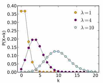
Poisson Probability Mass Function

The horizontal axis is the index k, the number of occurrences. The function is only defined at integer values of k. The connecting lines are only guides for the eye.