

/en/excel2000/creating-formulas/content/
Simple formulas have one mathematical operation. Complex formulas involve more than one mathematical operation.
The order of mathematical operations is important. If you enter a formula that contains several operations—like adding, subtracting, and dividing—Excel knows to work those operations in a specific order. The order of operations is:
1. Operations enclosed in parentheses
2. Exponential calculations (to the power of)
3. Multiplication and division, whichever comes first
4. Addition and subtraction, whichever comes first
Relative to the order, you will also calculate from left to right. Let's look at an example: 2*(6-4) =?
Is the answer 8 or 4? If you calculated in the order in which the numbers appear, ignoring the parentheses, 2*6-4, you'd get the wrong answer, 8. You must follow the order of operations to get the correct answer.
To calculate the correct answer:
1. Calculate the operation in parentheses: 6-4=2.
2. Multiply 2*2=4.
3. The answer is 4.
![]() When using formulas, the results change each time the numbers are edited.
When using formulas, the results change each time the numbers are edited.
![]() In Excel, never do math in your head and type the answer in a cell where you would expect to have a formula calculate the answer.
In Excel, never do math in your head and type the answer in a cell where you would expect to have a formula calculate the answer.
When you create a complex formula, Excel automatically follows the order of operations. If you want a certain portion of the formula to be calculated first, put it in parentheses—for example, =(B8+B9)*A10.
![]() Try changing one of the values in the formula and watch the answer to the formula change.
Try changing one of the values in the formula and watch the answer to the formula change.
Excel will not always tell you if your formula contains an error, so it's up to you to check all of your formulas. To learn how to do this, read the Double-Check Your Formulas lesson from our Excel Formulas tutorial.
Once you've created a working formula, don't waste time typing and retyping it. Simply fill it to the other cells. To do this, you will need to recognize the mouse pointer's various shapes. When you move the mouse pointer around the Excel window, it changes shape and function.
If you'll be copying a formula to a surrounding cell, you can use the Fill method. The square box in the lower-right corner of the cell pointer is the fill handle.
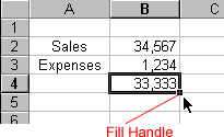
![]() In Excel, the references change as the formula is copied. Remember, you use references to identify cells containing the numbers you want to calculate in a formula.
In Excel, the references change as the formula is copied. Remember, you use references to identify cells containing the numbers you want to calculate in a formula.
![]() You can also use copy and paste to copy a formula to other cells. This will be discussed on the next page.
You can also use copy and paste to copy a formula to other cells. This will be discussed on the next page.
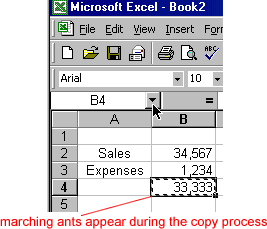
![]() Cut, copy, and paste are discussed in detail in our Office 2000 tutorial.
Cut, copy, and paste are discussed in detail in our Office 2000 tutorial.
If you entered an incorrect formula or added new data and need to change the formula to reflect the new entries, you can revise your formula using the range finder or your keyboard.
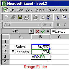

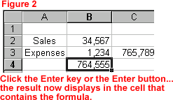
You can also select the cell that contains the formula, select the part of the formula you want to revise, and type a new cell address. This is a somewhat inaccurate method, though, because it's easy to mistype.
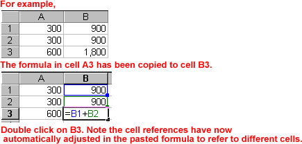
Typically, when you copy a formula that uses references, Excel automatically adjusts the reference in the pasted formula to refer to different cells relative to the position of the formula.
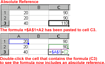
Sometimes when you copy a formula, you don't want one of the cell references to change. Creating an absolute reference—a reference to a cell that does not change when copying a formula—solves this problem. An absolute reference always refers to the same cell or range. It is designated in the formula by the dollar sign ($).
For this exercise, delete the original formulas and start again.
Knowing the order of operations is essential to getting the correct answer. Spend some time memorizing it:
1. Operations enclosed in parentheses
2. Exponential calculations (to the power of)
3. Multiplication and division, whichever comes first
4. Addition and subtraction, whichever comes first
/en/excel2000/formatting-numbers/content/