

/en/excel2013/relative-and-absolute-cell-references/content/
A function is a predefined formula that performs calculations using specific values in a particular order. Excel includes many common functions that can be useful for quickly finding the sum, average, count, maximum value, and minimum value for a range of cells. In order to use functions correctly, you'll need to understand the different parts of a function and how to create arguments to calculate values and cell references
In order to work correctly, a function must be written a specific way, which is called the syntax. The basic syntax for a function is the equals sign (=), the function name (SUM, for example), and one or more arguments. Arguments contain the information you want to calculate. The function in the example below would add the values of the cell range A1:A20.
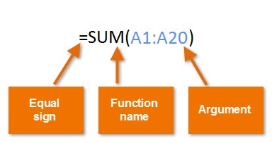 Syntax of a basic function
Arguments can refer to both individual cells and cell ranges and must be enclosed within parentheses. You can include one argument or multiple arguments, depending on the syntax required for the function.
For example, the function =AVERAGE(B1:B9) would calculate the average of the values in the cell range B1:B9. This function contains only one argument.
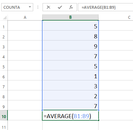 A function with a single argument
Multiple arguments must be separated by a comma. For example, the function =SUM(A1:A3, C1:C2, E1) will add the values of all the cells in the three arguments.
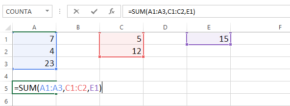 A function with multiple arguments
Excel has a variety of functions available. Here are some of the most common functions you'll use:
In our example below, we'll create a basic function to calculate the average price per unit for a list of recently ordered items using the AVERAGE function.
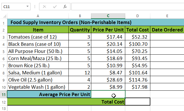 Selecting cell C11
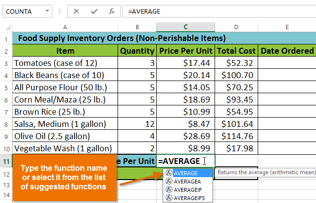 Entering the AVERAGE function
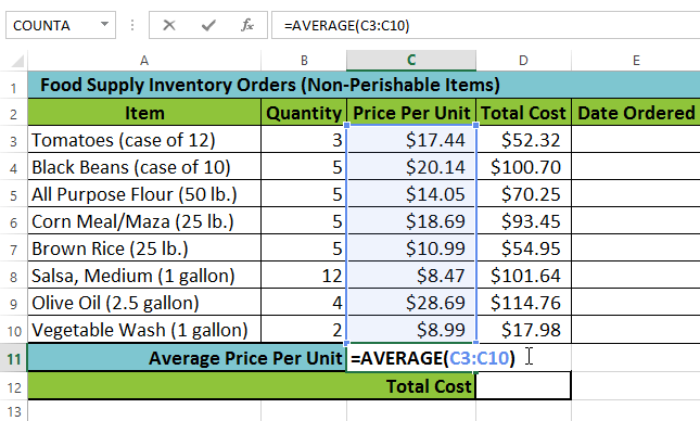 Creating an argument
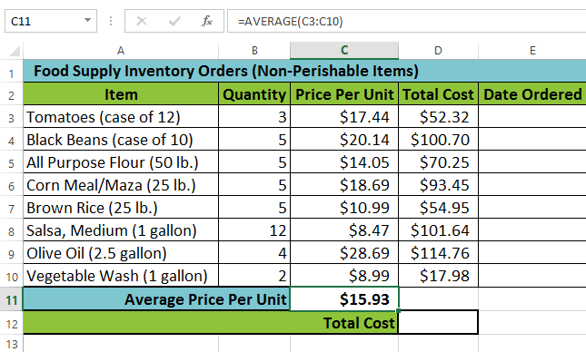 The completed function and calculated value
Excel will not always tell you if your formula contains an error, so it's up to you to check all of your formulas. To learn how to do this, read the Double-Check Your Formulas lesson from our Excel Formulas tutorial.
The AutoSum command allows you to automatically insert the most common functions into your formula, including SUM, AVERAGE, COUNT, MIN, and MAX. In our example below, we'll create a function to calculate the total cost for a list of recently ordered items using the SUM function.
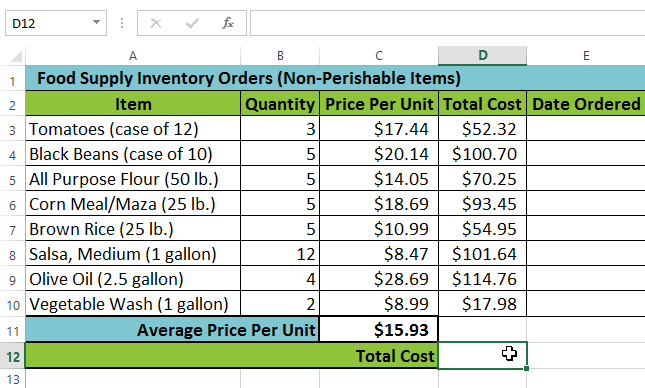 Selecting cell D12
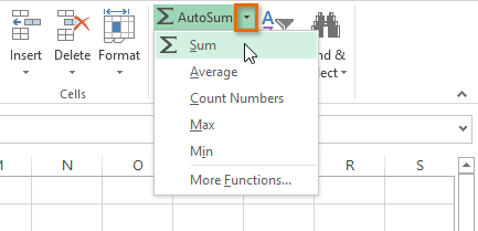 Selecting Sum from the AutoSum command drop-down menu
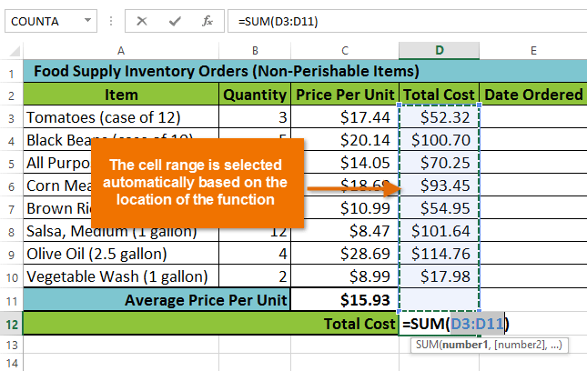 The inserted function and automatically selected cell range
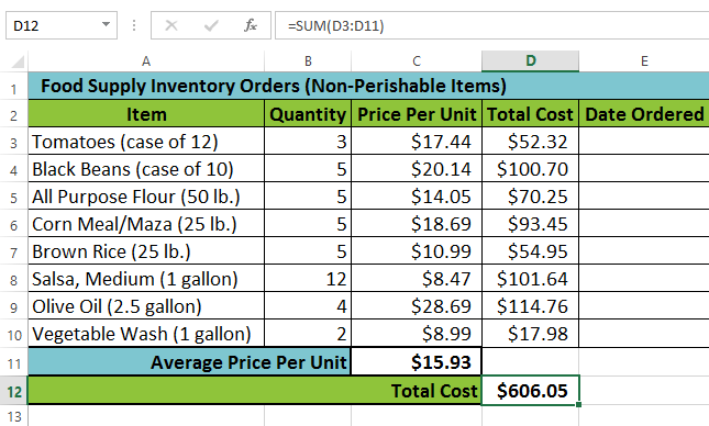 The completed function and calculated value
The AutoSum command can also be accessed from the Formulas tab on the Ribbon.
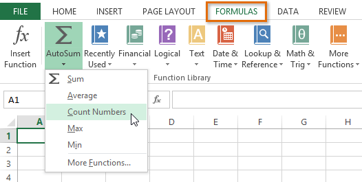 Accessing the AutoSum command from the Formulas tab
You can also use the Alt+= keyboard shortcut instead of the AutoSum command. To use this shortcut, hold down the Alt key and then press the equals sign.
Watch the video below to see this shortcut in action.
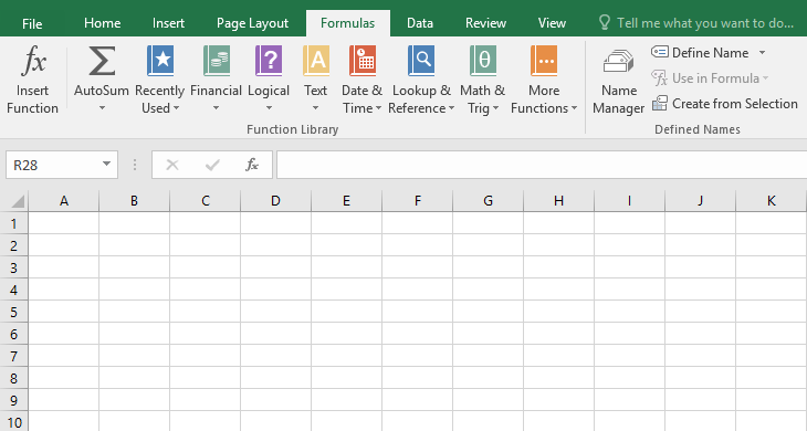
While there are hundreds of functions in Excel, the ones you use most frequently will depend on the type of data your workbooks contains. There is no need to learn every single function, but exploring some of the different types of functions will be helpful as you create new projects. You can search for functions by category, such as Financial, Logical, Text, Date & Time, and more from the Function Library on the Formulas tab.
 Clicking the Formulas tab
Click the buttons in the interactive below to learn more about the different types of functions in Excel.
In our example below, we'll use a function to calculate the number of business days it took to receive items after they were ordered. In our example, we'll use the dates in columns B and C to calculate the delivery time in column D.
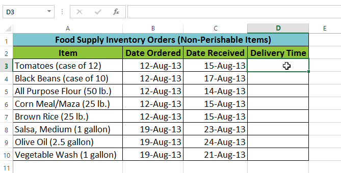 Selecting cell D3
 Selecting the Date & Time category from the Function Library
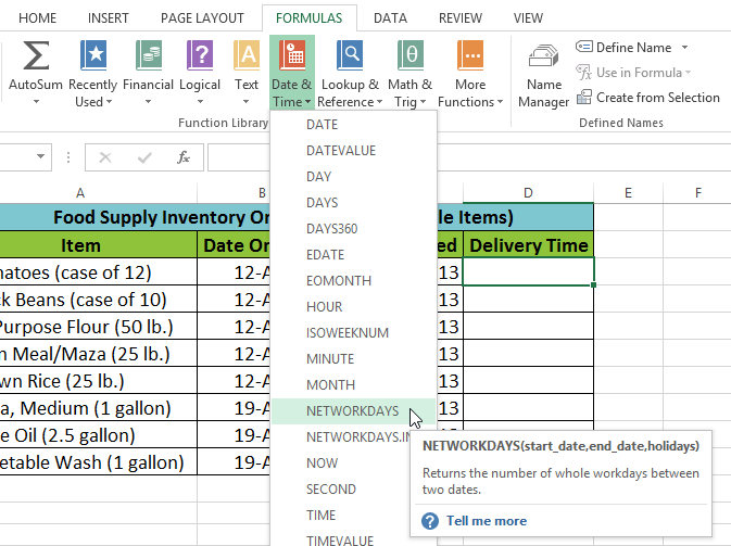 Selecting the NETWORKDAYS function
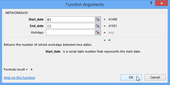 Clicking OK
 The completed function and calculated value
Like formulas, functions can be copied to adjacent cells. Hover the mouse over the cell that contains the function, then click, hold, and drag the fill handle over the cells you want to fill. The function will be copied, and values for those cells will be calculated relative to their rows or columns.
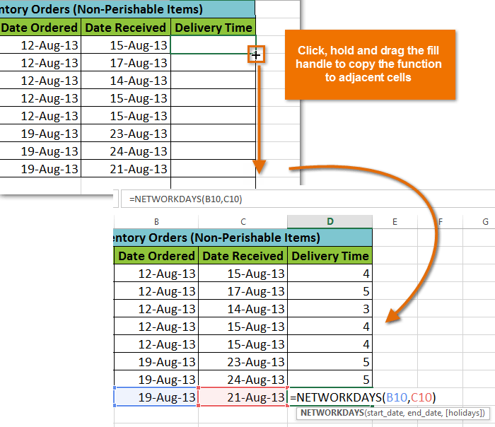 Copying a function to adjacent cells using the fill handle
If you're having trouble finding the right function, the Insert Function command allows you to search for functions using keywords. While it can be useful, this command is sometimes difficult to use. If you don't have much experience with functions, you may have more success browsing the Function Library instead. For more advanced users, however, the Insert Function command can be a powerful way to find a function quickly.
In our example below, we want to find a function that will count the total number of items ordered. We want to count the cells in the Item column, which uses text. We cannot use the basic COUNT function because it will only count cells with numerical information. Instead, we will need to find a function that counts the total number of cells within a cell range.
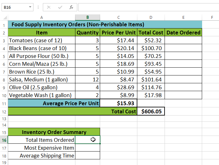 Selecting cell B16
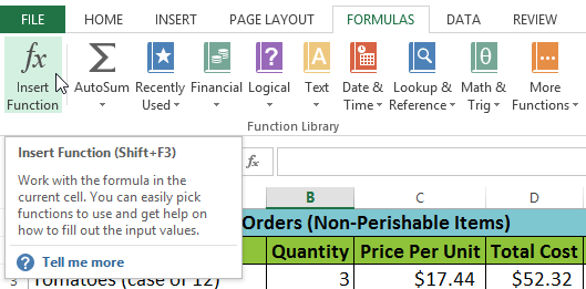 Selecting the Insert Function command
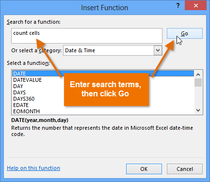 Searching for a function with keywords
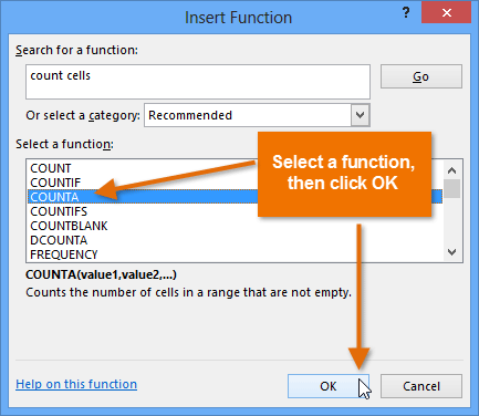 Selecting a function and clicking OK
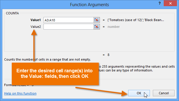 Entering an argument and clicking OK
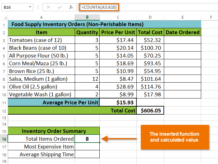 The completed function and calculated value
If you're comfortable with basic functions, you may want to try a more advanced one like VLOOKUP. You can check out our article on How to Use Excel's VLOOKUP Function for more information. If you want to learn even more about functions, check out our Excel Formulas tutorial.
/en/excel2013/freezing-panes-and-view-options/content/