/en/excelformulas/invoice-part-4-more-shipping-options/content/

Our spreadsheet

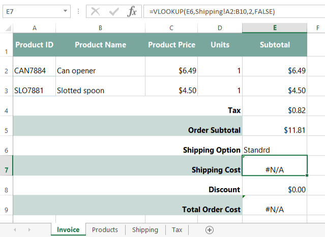
Once you've downloaded our spreadsheet, open the file in Excel or another spreadsheet application. Cell E7 is using the same VLOOKUP formula we added in Invoice, Part 4: More Shipping Options, but it's no longer pulling in the Shipping Cost correctly. And since the formula in cell E9 depends on that value, it's not able to calculate correctly either.

What are we trying to fix?

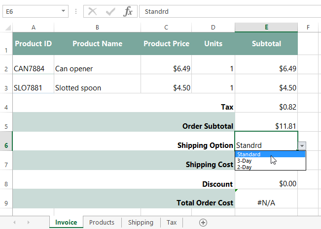
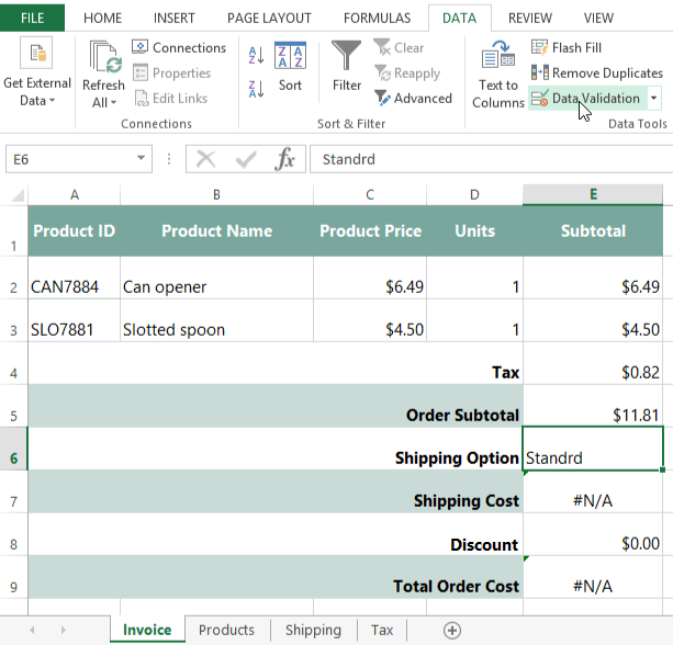
If we look at cell E6, we can see that the word Standard is misspelled. The Shipping worksheet doesn't contain the word "Standrd", so our VLOOKUP function doesn't return any results. While we could simply type in the correct spelling, that wouldn't prevent someone from making the same mistake in the future. To make sure this doesn't happen again, we can add data validation to our spreadsheet.

Data validation

Data validation allows you to control exactly what a user can enter into a cell. In our example, we can use data validation to ensure that the user chooses one of the three possible shipping options. To make things even easier, we can insert a drop-down list of the possible options.

This kind of data validation allows you to build a powerful, fool-proof spreadsheet. Since users won't have to type in data manually, the spreadsheet will be faster to use, and there's a much lower chance that someone can introduce an error. Depending on what spreadsheet program you're using, the process of adding data validation will vary. We'll show you how to add data validation in Microsoft Excel and Google Sheets.

Data validation in Excel

Since we already have a list of shipping options in the Shipping worksheet, we're going to tell Excel to use the data in that list to control which values a user can select. But before we do this, we'll actually need to name the cell range first. Naming cell ranges is one way to keep track of important cell ranges in your spreadsheet.

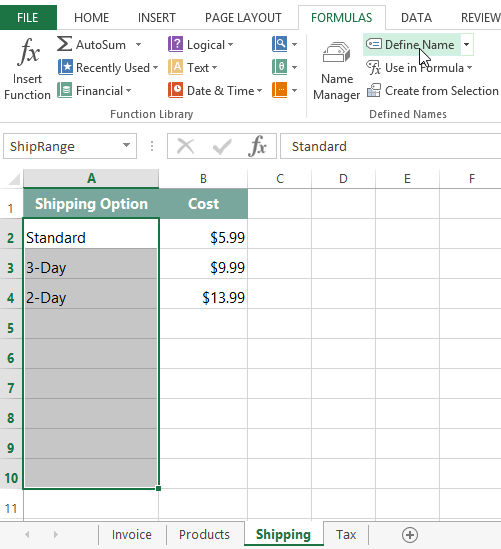
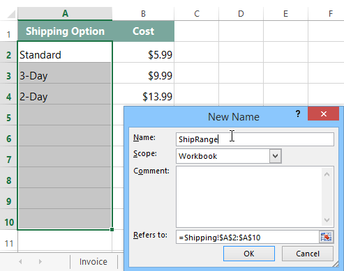
To name a cell range (Excel 2007-2019):

1. Select the cell range you wish to name. In this example, we'll select the cell range A2:A10 on the Shipping worksheet (we're including empty rows just in case more shipping options are added later on).
2. Go to the Formulas tab, and then click Define Name.

   
   

   
3. A dialog box will appear. Type a name for the cell range in the Name: field and then click OK. In our example, we'll name it ShipRange.
   
4. Click OK. The cell range will be named.

If you ever add more data to your spreadsheet, you can easily check all of your named ranges with the Name Manager to make sure they are including all of the data.

To create a data validation drop-down list (Excel 2007-2019):

1. Select the cell where you want the drop-down list to appear. In our example, that's cell E6 on the Invoice worksheet.
2. On the Data tab, click the Data Validation command.
   
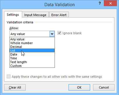
3. A dialog box will appear. In the Allow: field, select List.
   
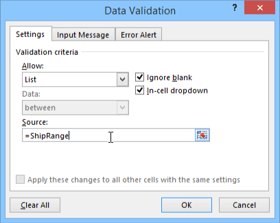
4. In the Source: field, type the equals sign (=) and the name of your range, and then click OK. In our example, we'll type: =ShipRange.
   
5. A drop-down arrow will appear next to the selected cell. Click the arrow to select the desired option. In our example, we'll select Standard. Alternatively, you can type the shipping option, but Excel will only accept it if it is spelled correctly.

   
   

   
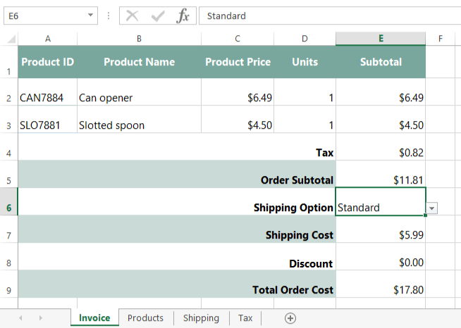
6. The selected value will appear in the cell. Now that we're searching for the exact name of a shipping option, our VLOOKUP function is working correctly again.
   

Data validation with Google Sheets

Creating a drop-down list for Google Sheets is actually a little simpler than Excel, because you don't need to name a cell range beforehand.

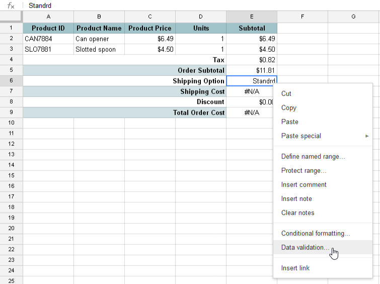
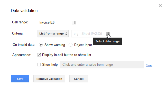
To create a data validation drop-down list (Google Sheets):

1. Right-click the cell where you want the drop-down list to appear and select Data validation. In our example, we'll select cell E6.
   
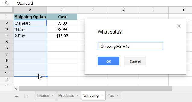
2. A dialog box will appear. Click Select data range in the Criteria: field.
   
3. Select the data that will appear in the drop-down list, and then click OK. In our example, the shipping options are stored in cell range A2:A4 on the Shipping worksheet, but we'll select A2:A10 (we're including empty rows just in case more shipping options are added later on).
   
4. Click Save to close the dialog box.
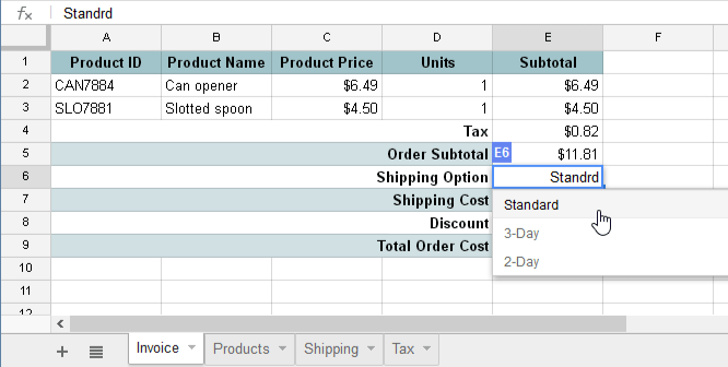
5. A drop-down arrow will appear within the selected cell. Click the arrow to select the desired option. In our example, we'll select Standard. Alternatively, you can type the shipping option, but Google Sheets will only accept it if it is spelled correctly.
   
6. The selected value will appear in the cell.

There we go—with our new data validation drop-down list, it'll be a lot harder for someone to break our function in the future!

/en/excelformulas/excel-formulas-quiz/content/