Bertrand competition
Bertrand competition is a model of competition used in economics, named after Joseph Louis François Bertrand (1822–1900). It describes interactions among firms (sellers) that set prices and their customers (buyers) that choose quantities at the prices set. The model was formulated in 1883 by Bertrand in a review of Antoine Augustin Cournot's book Recherches sur les Principes Mathématiques de la Théorie des Richesses (1838) in which Cournot had put forward the Cournot model.[1] Cournot's model argued that each firm should maximise its profit by selecting a quantity level and then adjusting price level to sell that quantity. The outcome of the model equilibrium involved firms pricing above marginal cost; hence, the competitive price. In his review, Bertrand argued that each firm should instead maximise its profits by selecting a price level that undercuts its competitors' prices, when their prices exceed marginal cost.[2] The model was not formalized by Bertrand; however, the idea was developed into a mathematical model by Francis Ysidro Edgeworth in 1889.[3]
Underlying assumptions of Bertrand competition
Considering the simple framework, the underlying assumptions that the Bertrand model makes is as follows:
- there are firms () competing in the market that produce homogenous goods; that is, identical products;[4]
- the market demand function , where Q is the summation of quantity produced by firms , is continuous and downward sloping with [5];
- the marginal cost is symmetric, [6];
- it is a static game; firms simultaneously set price, without knowing the other firm's decision;[5] and
- firms don't have a capacity constraint; that is, each firm has the capability to produce enough goods to meet market demand.[7]
Furthermore, it is intuitively deducible, when considering the law of demand of firms' competition in the market:
The Bertrand duopoly equilibrium
Why is the competitive price a Nash equilibrium in the Bertrand model? First, if both firms set the competitive price with price equal to marginal cost (unit cost), neither firm will earn any profits. However, if one firm sets price equal to marginal cost, then if the other firm raises its price above unit cost, then it will earn nothing, since all consumers will buy from the firm still setting the competitive price (recall that it is willing to meet unlimited demand at price equals unit cost even though it earns no profit). No other price is an equilibrium. If both firms set the same price above unit cost and share the market, then each firm has an incentive to undercut the other by an arbitrarily small amount and capture the whole market and almost double its profits. So there can be no equilibrium with both firms setting the same price above marginal cost. This is due to the firms competing over goods and services that are considered substitutes; that is, consumers having identical preferences towards each product and only preferring the cheaper of the two. Also, there can be no equilibrium with firms setting different prices. The firms setting the higher price will earn nothing (the lower priced firm serves all of the customers). Hence the higher priced firm will want to lower its price to undercut the lower-priced firm. Hence the only equilibrium in the Bertrand model occurs when both firms set price equal to unit cost (the competitive price).[9]
Note that the Bertrand equilibrium is a weak Nash-equilibrium. The firms lose nothing by deviating from the competitive price: it is an equilibrium simply because each firm can earn no more than zero profits given that the other firm sets the competitive price and is willing to meet all demand at that price.
Classic modelling of the Bertrand competition
The Bertrand model of price competition in a duopoly market producing homogenous goods has the following characteristics:
- Players: Two firms with constant marginal cost ;
- Strategic Variables: Firm's select the price level (i.e., );
- Timing: Simultaneous move game;
- Firm Payoffs: Profit; and
- Information: Complete.[5]
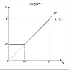
 Best response of firm 1 plotted as a function of firm 2's price
Firm ’s individual demand function is downward sloping and a function of the price set by each firm:[9]
Important to note, in this case, the market demand is continuous; however, the firm's demand is discontinuous, as seen in the above function statement. This means the firm's profit function is also discontinuous.[5] Therefore, firm aims to maximise its profit, as stated below, taking as given:[10]
In order to derive the best response for firm , let be the monopoly price that maximises total industry profit, where . This highlights the incentive for firms to 'undercut' rival firms. As if the rival sets the price at firm can reduce its price by the smallest currency unit, , to capture the entire market demand, .[10] Therefore, firm ’s best response is:[5]

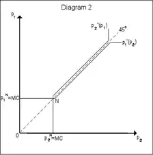
Diagram 1 illustrates firm 1's best response function, , given the price set by firm 2. Note, in the diagram stands for marginal cost, . The Nash Equilibrium () in the Bertrand model is the mutual best response; an equilibrium where neither firm has an incentive to deviate from it. As illustrated in the Diagram 2, the Bertrand-Nash equilibrium occurs when the best response function for both firm's intersects at the point, where . This means both firms make zero economic profits.[5]
Therefore, if rival prices below marginal cost, firm ends up making losses attracting extra demand and is better of setting price level to marginal cost. Important to note, Bertrand's model of price competition leads to a perfect competitive outcome.[7] This is known as the Bertrand paradox; as two competitors in a market are sufficient to generate competitive pricing; however, this result is not consistent in many real world industries.[5]
If one firm has lower average cost (a superior production technology), it will charge the highest price that is lower than the average cost of the other one (i.e. a price just below the lowest price the other firm can manage) and take all the business. This is known as "limit pricing".
Critical analysis of the Bertrand model
The Bertrand model rests on some very extreme assumptions. For example, it assumes that consumers want to buy from the lowest priced firm. There are various reasons why this may not hold in many markets: non-price competition and product differentiation, transport and search costs. For example, would someone travel twice as far to save 1% on the price of their vegetables? The Bertrand model can be extended to include product or location differentiation but then the main result – that price is driven down to marginal cost – no longer holds. With search costs, there may be other equilibria apart from the competitive price – the monopoly price or even price dispersion may be equilibria as in the classic "Bargains and Rip-offs" model.[11]
The model also ignores capacity constraints. If a single firm does not have the capacity to supply the whole market then the "price equals marginal cost" result may not hold. The analysis of this case was started by Francis Ysidro Edgeworth and has become known as the Bertrand–Edgeworth model. With capacity constraints, there may not exist any pure strategy Nash equilibrium, the so-called Edgeworth paradox. However, in general there will exist a mixed-strategy Nash equilibrium as shown by Huw Dixon.[12]
Moreover, some economists have criticized the model as leading to impractical outcomes in situations, where firms have fixed cost and, as mentioned previously, constant marginal cost, . Hence, the total cost, , of producing units is, . As described in the classic model, prices eventually are driven down to marginal cost, where firms are making zero economic profit and earn no margins on inframarginal units. Thus, firms are not able to recouple any fixed costs. However, if firms have an upward-sloping marginal cost curve, they can earn marginal on infra-marginal sales, which contributes to recouping fixed costs.[7]
There is a big incentive to cooperate in the Bertrand model; colluding to charge the monopoly price, , and sharing the market equally, , where is the number of firms in the market.[13] However, not colluding and charging marginal cost is the non-cooperative outcome and the only Nash equilibrium of this model.[7] Therefore, moving from a simultaneous move game to a repeated game with infinite horizon, then collusion is possible because of the Folk Theorem.[14]
Bertrand competition versus Cournot competition
The Bertrand and Cournot model focus on different aspects of the competitive process, which has led to the model identifying different set of mechanisms that vary the characteristics of the market demand that are exhibited by the firms. Cournot model assumes that the market allocates sales equal to whatever any given firm quantity produced, but at the price level determined by the market. Whereas the Bertrand model assumes that the firm with the lowest price acquires all the sales in the market.[2]
When comparing the models, the oligopoly theory suggest that the Bertrand industries are more competitive than Cournot industries. This is because quantities in the Cournot model are considered as strategic substitutes; that is, the increase in quantity level produced by a firm is accommodated by the rival, producing less. Whereas the prices in the Bertrand model are strategic complements; a firm aggressively counters an increase in price level by reducing its price below the rivals.[15]
Moreover, both models are criticised based on the assumptions that are made in comparison to the real-world scenario. However, the results from the classic models can be reconciled in a manner of thinking, as presented below. Considering the models appropriate application in the market:
- Cournot model is applicable in markets where the firm must make production decision in advance and must be committed to selling that quantity level; thus, unlikely to react to fluctuations in rival's quantity produced.
- Bertrand model is applicable in markets where capacity is sufficiently flexible and firms are capable to meet any market demand that arises at price level, which they set.[16]
Neither model is necessarily "better" than the other. The accuracy of the predictions of each model will vary from industry to industry, depending on the closeness of each model to the industry situation. If capacity and output can be easily changed, Bertrand is generally a better model of duopoly competition. If output and capacity are difficult to adjust, then Cournot is generally a better model.
Under some conditions the Cournot model can be recast as a two-stage model, wherein the first stage firms choose capacities, and in the second they compete in Bertrand fashion.
Bertrand Competition in Real Life
Bertrand Competition with Asymmetric Marginal Costs
In Bertrand Competition, we have made several assumptions, for instance, each firm produces identical goods and cost. However, this is not the case in the real world because there are a lot of factors that lead the cost of different firms to become slightly different like the cost of renting and the larger scale of the firm can enjoy economies of scale. Thus, different researchers tried to investigate the result of Bertrand Competition with asymmetric marginal cost. According to the experiment from “Bertrand competition with asymmetric costs: Experimental evidence”, the author found that there is a negative relationship between the level of asymmetry in the cost and the price set by the firms (J Boone, et al., 2012).[17] It means that firms have different incentives to set their prices.
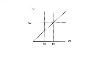
Thomas Demuynck et al. (2019) conducted research to find out a solution in pure strategies in Bertrand competition with asymmetric costs.[18] Ha has defined the Myopic Stable Set (MSS)for Normal-form games. Suppose there are two firms, we use C for the marginal cost, C1 stands for the marginal cost of firm 1 and C2 stands for the marginal cost of firm 2. From the result, there are two cases:

- C1 = C2 = C
This is the case of the basic Bertrand Competition which both firms have the same marginal cost. From the figure, MSS has illustrated that there is only one unique point that both firms are going to set their price. It is the pure strategy of Nash equilibrium.
- C1 < C2
It means that the marginal cost of Firm 2 is higher than the marginal cost of Firm 1. Under this situation, firm 2 can only set their price equal to their marginal cost. On the other hand, Firm 1 can choose its price between its marginal cost and Firm 2's marginal cost. Thus, there are a lot of points for Firm 1 to set its price.
As you can see, Firms may not set their price equal to their marginal cost under asymmetric costs, unlike the standard Bertrand Competition Model. From the situation, firms with the lower marginal cost can choose whatever they want within the range between their marginal cost and other firms’ marginal costs. There is no absolute answer to which price they should set, it is just based on different factors, for example, the current market situation.
At the same time, Subhasish Dugar et al. (2009) conducted research about the relationship between the size of cost asymmetry and Bertrand Competition.[19] They found that there is no huge difference when the cost asymmetry is small as there is relatively little impact on competition. However, the lower-cost firm will undercut the price and capture a large market share when the size of cost asymmetry is large.
Bertrand Competition with Network effects
Also, the standard Bertrand Competition also assumes that all consumers will choose the product from the firm with a lower price and the firm can only set their price based on their marginal costs. However, it is not perfectly correct as the theory did not mention the network effects. Consumers will buy a product based on the number of other consumers using it. It is very rational, like when you purchase sports shoes, most of us will prefer Nike and Adidas. As they are relatively huge brands and both of them have a strong customer network, we will have a certain confidence guarantee with many people are using their products.
However, Christian and Irina (2008)found a different result if the market has a network effects.[20] Firms will prefer to set their price aggressively in order to attract more customers and increase the company network. Masaki (2018) also mentioned firms can gain a larger customer base by setting their prices aggressively and they will attract more and more customers through network effects.[21] It creates a positive feedback loop. As you can see, firms are not only setting their price blindly but also willing to gain a larger customer network.
See also
References
- Bertrand, J. (1883) "Book review of theorie mathematique de la richesse sociale and of recherches sur les principles mathematiques de la theorie des richesses", Journal de Savants 67: 499–508
- Qin, Cheng-Zhong; Stuart, Charles (1997). "Bertrand versus Cournot Revisited". Economic Theory. 10 (3): 497–507. doi:10.1007/s001990050169. ISSN 0938-2259. JSTOR 25055054. S2CID 153431949.
- Edgeworth, Francis (1889) “The pure theory of monopoly”, reprinted in Collected Papers relating to Political Economy 1925, vol.1, Macmillan.
- Dastidar, Krishnendu Ghosh (1995). "On the Existence of Pure Strategy Bertrand Equilibrium". Economic Theory. 5 (1): 20. doi:10.1007/BF01213642. JSTOR 25054821. S2CID 153890403 – via JSTOR.
- Tremblay, Carol Horton; Tremblay, Victor J. (2019). "Oligopoly Games and the Cournot–Bertrand Model: A Survey". Journal of Economic Surveys. 33 (5): 1555–1577. doi:10.1111/joes.12336. ISSN 0950-0804. S2CID 202322675.
- Bian, Junsong; Lai, Kin Keung; Hua, Zhongsheng; Zhao, Xuan; Zhou, Guanghui (2018-10-01). "Bertrand vs. Cournot competition in distribution channels with upstream collusion". International Journal of Production Economics. 204: 278–289. doi:10.1016/j.ijpe.2018.08.007. ISSN 0925-5273. S2CID 158245642.
- Bhattacharya, Rajeev; Sherry, Edward F. (2016). "Bertrand Competition". The Palgrave Encyclopedia of Strategic Management. pp. 1–2. doi:10.1057/978-1-349-94848-2_571-1. ISBN 978-1-349-94848-2. S2CID 219346516.
- Petrosyan, Leon A; Mazalov, Vladimir V; Zenkevich, Nikolay A, eds. (2018). Frontiers of Dynamic Games. Static & Dynamic Game Theory: Foundations & Applications. doi:10.1007/978-3-319-92988-0. ISBN 978-3-319-92987-3. S2CID 239449242.
- Narahari, Y.; Garg, Dinesh; Narayanam, Ramasuri; Prakash, Hastagiri (2009), Game Theoretic Problems in Network Economics and Mechanism Design Solutions, Springer, p. 21, ISBN 978-1-84800-937-0
- Dastidar, Krishnendu Ghosh (1995). "On the Existence of Pure Strategy Bertrand Equilibrium". Economic Theory. 5 (1): 19–32. doi:10.1007/BF01213642. ISSN 0938-2259. JSTOR 25054821. S2CID 153890403.
- Salop, S.; Stiglitz, J. (1977). "Bargains and Ripoffs: A Model of Monopolistically Competitive Price Dispersion". The Review of Economic Studies. 44 (3): 493–510. doi:10.2307/2296903. JSTOR 2296903.
- Dixon, H. (1984). "The existence of mixed-strategy equilibria in a price-setting oligopoly with convex costs". Economics Letters. 16 (3–4): 205–212. doi:10.1016/0165-1765(84)90164-2.
- Cramton, Peter C.; Palfrey, Thomas R. (1990). "Cartel Enforcement with Uncertainty about Costs". International Economic Review. 31 (1): 17–47. doi:10.2307/2526626. ISSN 0020-6598. JSTOR 2526626.
- Fudenberg, Drew; Maskin, Eric (1986). "The Folk Theorem in Repeated Games with Discounting or with Incomplete Information". Econometrica. 54 (3): 533–554. doi:10.2307/1911307. ISSN 0012-9682. JSTOR 1911307.
- Brander, James A.; Spencer, Barbara J. (February 2015). "Endogenous Horizontal Product Differentiation under Bertrand and Cournot Competition: Revisiting the Bertrand Paradox". Working Paper Series. doi:10.3386/w20966. S2CID 153281771.
{{cite journal}}: Cite journal requires|journal=(help) - Kirui, Benard Kipyegon (2013). "Reconciling Cournot and Bertrand Outcomes: A Review". University of Dar Es Salaam, Dar Es Salaam: 3–7. hdl:10419/97305 – via EconStor.
- Boone, Jan; Larraín Aylwin, María Jose; Müller, Wieland; Ray Chaudhuri, Amrita (2012-10-01). "Bertrand competition with asymmetric costs: Experimental evidence". Economics Letters. 117 (1): 134–137. doi:10.1016/j.econlet.2012.04.098. ISSN 0165-1765.
- Demuynck, Thomas; Herings, P. Jean-Jacques; Saulle, Riccardo D.; Seel, Christian (2019-09-01). "Bertrand competition with asymmetric costs: a solution in pure strategies". Theory and Decision. 87 (2): 147–154. doi:10.1007/s11238-019-09698-4. ISSN 1573-7187. S2CID 255111873.
- Dugar, Subhasish; Mitra, Arnab (2009-08-23). "The Size of the Cost Asymmetry and Bertrand Competition: Experimental Evidence". Rochester, NY. doi:10.2139/ssrn.1328662. S2CID 153834493. SSRN 1328662.
{{cite journal}}: Cite journal requires|journal=(help) - Suleymanova, Irina; Wey, Christian (2011-09-18). "Bertrand Competition in Markets with Network Effects and Switching Costs". The B.E. Journal of Economic Analysis & Policy. 11 (1). doi:10.2202/1935-1682.2359. ISSN 1935-1682. S2CID 1742340.
- Aoyagi, Masaki (2018-11-01). "Bertrand competition under network externalities". Journal of Economic Theory. 178: 517–550. doi:10.1016/j.jet.2018.10.006. ISSN 0022-0531.