Feedforward neural network
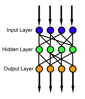
A feedforward neural network (FNN) is one of the two broad types of artificial neural network, characterized by direction of the flow of information between its layers.[2] Its flow is uni-directional, meaning that the information in the model flows in only one direction—forward—from the input nodes, through the hidden nodes (if any) and to the output nodes, without any cycles or loops,[2] in contrast to recurrent neural networks,[3] which have a bi-directional flow. Modern feedforward networks are trained using the backpropagation method[4][5][6][7][8] and are colloquially referred to as the "vanilla" neural networks.[9]
| Part of a series on |
| Machine learning and data mining |
|---|
 |

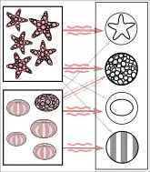
In reality, textures and outlines would not be represented by single nodes, but rather by associated weight patterns of multiple nodes.
Timeline
- In 1958, a layered network of perceptrons, consisting of an input layer, a hidden layer with randomized weights that did not learn, and an output layer with learning connections, was introduced already by Frank Rosenblatt in his book Perceptron.[10][11][12] This extreme learning machine[13][12] was not yet a deep learning network.
- In 1965, the first deep-learning feedforward network, not yet using stochastic gradient descent, was published by Alexey Grigorevich Ivakhnenko and Valentin Lapa, at the time called the Group Method of Data Handling.[14][15][12]
- In 1967, a deep-learning network, using stochastic gradient descent for the first time, was able to classify non-linearily separable pattern classes, as reported Shun'ichi Amari.[16] Amari's student Saito conducted the computer experiments, using a five-layered feedforward network with two learning layers.
- In 1970, modern backpropagation method, an efficient application of a chain-rule-based supervised learning,[17][18] was for the first time published by the Finnish researcher Seppo Linnainmaa.[4][19][12] The term (i.e. "back-propagating errors") itself has been used by Rosenblatt himself,[11] but he did not know how to implement it,[12] although a continuous precursor of backpropagation was already used in the context of control theory in 1960 by Henry J. Kelley.[5][12] It is known also as a reverse mode of automatic differentiation.
- In 1982, backpropagation was applied in the way that has become standard, for the first time by Paul Werbos.[7][12]
- In 1985, an experimental analysis of the technique was conducted by David E. Rumelhart et al..[8] Many improvements to the approach have been made in subsequent decades.[12]
- In 1987, using a stochastic gradient descent within a (wide 12-layer nonlinear) feed-forward network, Matthew Brand has trained it to reproduce logic functions of nontrivial circuit depth, using small batches of random input/output samples. He, however, concluded that on hardware (sub-megaflop computers) available at the time it was impractical, and proposed using fixed random early layers as an input hash for a single modifiable layer.[20]
- In 1990s, an (much simpler) alternative to using neural networks, although still related[21] support vector machine approach was developed by Vladimir Vapnik and his colleagues. In addition to performing linear classification, they were able to efficiently perform a non-linear classification using what is called the kernel trick, using high-dimensional feature spaces.
- In 2003, interest in backpropagation networks returned due to the successes of deep learning being applied to language modelling by Yoshua Bengio with co-authors.[22]
- In 2017, modern transformer architectures has been introduced.[23]
- In 2021, a very simple NN architecture combining two deep MLPs with skip connections and layer normalizations was designed and called MLP-Mixer; its realizations featuring 19 to 431 millions of parameters were shown to be comparable to vision transformers of similar size on ImageNet and similar image classification tasks.[24]
Mathematical foundations
Activation function
The two historically common activation functions are both sigmoids, and are described by
- .
The first is a hyperbolic tangent that ranges from -1 to 1, while the other is the logistic function, which is similar in shape but ranges from 0 to 1. Here is the output of the th node (neuron) and is the weighted sum of the input connections. Alternative activation functions have been proposed, including the rectifier and softplus functions. More specialized activation functions include radial basis functions (used in radial basis networks, another class of supervised neural network models).
In recent developments of deep learning the rectified linear unit (ReLU) is more frequently used as one of the possible ways to overcome the numerical problems related to the sigmoids.
Learning
Learning occurs by changing connection weights after each piece of data is processed, based on the amount of error in the output compared to the expected result. This is an example of supervised learning, and is carried out through backpropagation.
We can represent the degree of error in an output node in the th data point (training example) by , where is the desired target value for th data point at node , and is the value produced at node when the th data point is given as an input.
The node weights can then be adjusted based on corrections that minimize the error in the entire output for the th data point, given by
- .
Using gradient descent, the change in each weight is
where is the output of the previous neuron , and is the learning rate, which is selected to ensure that the weights quickly converge to a response, without oscillations. In the previous expression, denotes the partial derivate of the error according to the weighted sum of the input connections of neuron .
The derivative to be calculated depends on the induced local field , which itself varies. It is easy to prove that for an output node this derivative can be simplified to
where is the derivative of the activation function described above, which itself does not vary. The analysis is more difficult for the change in weights to a hidden node, but it can be shown that the relevant derivative is
- .
This depends on the change in weights of the th nodes, which represent the output layer. So to change the hidden layer weights, the output layer weights change according to the derivative of the activation function, and so this algorithm represents a backpropagation of the activation function.[25]
History
Linear neural network
The simplest kind of feedforward neural network is a linear network, which consists of a single layer of output nodes; the inputs are fed directly to the outputs via a series of weights. The sum of the products of the weights and the inputs is calculated in each node. The mean squared errors between these calculated outputs and a given target values are minimized by creating an adjustment to the weights. This technique has been known for over two centuries as the method of least squares or linear regression. It was used as a means of finding a good rough linear fit to a set of points by Legendre (1805) and Gauss (1795) for the prediction of planetary movement.[26][27][28][12][29]
Perceptron
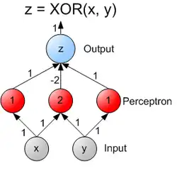
If using a threshold, i.e. a linear activation function, the resulting linear threshold unit is called a perceptron. (Often the term is used to denote just one of these units.) Multiple parallel linear units are able to approximate any continuous function from a compact interval of the real numbers into the interval [−1,1] despite the limited computational power of single unit with a linear threshold function. This result can be found in Peter Auer, Harald Burgsteiner and Wolfgang Maass "A learning rule for very simple universal approximators consisting of a single layer of perceptrons".[30]
Perceptrons can be trained by a simple learning algorithm that is usually called the delta rule. It calculates the errors between calculated output and sample output data, and uses this to create an adjustment to the weights, thus implementing a form of gradient descent.
Multilayer perceptron

A multilayer perceptron (MLP) is a misnomer for a modern feedforward artificial neural network, consisting of fully connected neurons with a nonlinear kind of activation function, organized in at least three layers, notable for being able to distinguish data that is not linearly separable.[31] It is a misnomer because the original perceptron used a Heaviside step function, instead of a nonlinear kind of activation function (used by modern networks).
Other feedforward networks
Examples of other feedforward networks include convolutional neural networks and radial basis function networks, which use a different activation function.
See also
References
- Ferrie, C., & Kaiser, S. (2019). Neural Networks for Babies. Sourcebooks. ISBN 1492671207.
{{cite book}}: CS1 maint: multiple names: authors list (link) - Zell, Andreas (1994). Simulation Neuronaler Netze [Simulation of Neural Networks] (in German) (1st ed.). Addison-Wesley. p. 73. ISBN 3-89319-554-8.
- Schmidhuber, Jürgen (2015-01-01). "Deep learning in neural networks: An overview". Neural Networks. 61: 85–117. arXiv:1404.7828. doi:10.1016/j.neunet.2014.09.003. ISSN 0893-6080. PMID 25462637. S2CID 11715509.
- Linnainmaa, Seppo (1970). The representation of the cumulative rounding error of an algorithm as a Taylor expansion of the local rounding errors (Masters) (in Finnish). University of Helsinki. p. 6–7.
- Kelley, Henry J. (1960). "Gradient theory of optimal flight paths". ARS Journal. 30 (10): 947–954. doi:10.2514/8.5282.
- Rosenblatt, Frank. x. Principles of Neurodynamics: Perceptrons and the Theory of Brain Mechanisms. Spartan Books, Washington DC, 1961
- Werbos, Paul (1982). "Applications of advances in nonlinear sensitivity analysis" (PDF). System modeling and optimization. Springer. p. 762–770. Archived (PDF) from the original on 14 April 2016. Retrieved 2 July 2017.
- Rumelhart, David E., Geoffrey E. Hinton, and R. J. Williams. "Learning Internal Representations by Error Propagation". David E. Rumelhart, James L. McClelland, and the PDP research group. (editors), Parallel distributed processing: Explorations in the microstructure of cognition, Volume 1: Foundation. MIT Press, 1986.
- Hastie, Trevor. Tibshirani, Robert. Friedman, Jerome. The Elements of Statistical Learning: Data Mining, Inference, and Prediction. Springer, New York, NY, 2009.
- Rosenblatt, Frank (1958). "The Perceptron: A Probabilistic Model For Information Storage And Organization in the Brain". Psychological Review. 65 (6): 386–408. CiteSeerX 10.1.1.588.3775. doi:10.1037/h0042519. PMID 13602029. S2CID 12781225.
- Rosenblatt, Frank (1962). Principles of Neurodynamics. Spartan, New York.
- Schmidhuber, Juergen (2022). "Annotated History of Modern AI and Deep Learning". arXiv:2212.11279 [cs.NE].
- Huang, Guang-Bin; Zhu, Qin-Yu; Siew, Chee-Kheong (2006). "Extreme learning machine: theory and applications". Neurocomputing. 70 (1): 489–501. CiteSeerX 10.1.1.217.3692. doi:10.1016/j.neucom.2005.12.126. S2CID 116858.
- Ivakhnenko, A. G. (1973). Cybernetic Predicting Devices. CCM Information Corporation.
- Ivakhnenko, A. G.; Grigorʹevich Lapa, Valentin (1967). Cybernetics and forecasting techniques. American Elsevier Pub. Co.
- Amari, Shun'ichi (1967). "A theory of adaptive pattern classifier". IEEE Transactions. EC (16): 279-307.
- Rodríguez, Omar Hernández; López Fernández, Jorge M. (2010). "A Semiotic Reflection on the Didactics of the Chain Rule". The Mathematics Enthusiast. 7 (2): 321–332. doi:10.54870/1551-3440.1191. S2CID 29739148. Retrieved 2019-08-04.
- Leibniz, Gottfried Wilhelm Freiherr von (1920). The Early Mathematical Manuscripts of Leibniz: Translated from the Latin Texts Published by Carl Immanuel Gerhardt with Critical and Historical Notes (Leibniz published the chain rule in a 1676 memoir). Open court publishing Company. ISBN 9780598818461.
- Linnainmaa, Seppo (1976). "Taylor expansion of the accumulated rounding error". BIT Numerical Mathematics. 16 (2): 146–160. doi:10.1007/bf01931367. S2CID 122357351.
- Matthew Brand (1988) Machine and Brain Learning. University of Chicago Tutorial Studies Bachelor's Thesis, 1988. Reported at the Summer Linguistics Institute, Stanford University, 1987
- R. Collobert and S. Bengio (2004). Links between Perceptrons, MLPs and SVMs. Proc. Int'l Conf. on Machine Learning (ICML).
- Bengio, Yoshua; Ducharme, Réjean; Vincent, Pascal; Janvin, Christian (March 2003). "A neural probabilistic language model". The Journal of Machine Learning Research. 3: 1137–1155.
- Geva, Mor; Schuster, Roei; Berant, Jonathan; Levy, Omer (2021). "Transformer Feed-Forward Layers Are Key-Value Memories". Proceedings of the 2021 Conference on Empirical Methods in Natural Language Processing. pp. 5484–5495. doi:10.18653/v1/2021.emnlp-main.446. S2CID 229923720.
- "Papers with Code - MLP-Mixer: An all-MLP Architecture for Vision".
- Haykin, Simon (1998). Neural Networks: A Comprehensive Foundation (2 ed.). Prentice Hall. ISBN 0-13-273350-1.
- Mansfield Merriman, "A List of Writings Relating to the Method of Least Squares"
- Stigler, Stephen M. (1981). "Gauss and the Invention of Least Squares". Ann. Stat. 9 (3): 465–474. doi:10.1214/aos/1176345451.
- Bretscher, Otto (1995). Linear Algebra With Applications (3rd ed.). Upper Saddle River, NJ: Prentice Hall.
- Stigler, Stephen M. (1986). The History of Statistics: The Measurement of Uncertainty before 1900. Cambridge: Harvard. ISBN 0-674-40340-1.
- Auer, Peter; Harald Burgsteiner; Wolfgang Maass (2008). "A learning rule for very simple universal approximators consisting of a single layer of perceptrons" (PDF). Neural Networks. 21 (5): 786–795. doi:10.1016/j.neunet.2007.12.036. PMID 18249524. Archived from the original (PDF) on 2011-07-06. Retrieved 2009-09-08.
- Cybenko, G. 1989. Approximation by superpositions of a sigmoidal function Mathematics of Control, Signals, and Systems, 2(4), 303–314.

