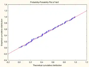
P–P plot

A P–P plot plots two cumulative distribution functions (cdfs) against each other:[1] given two probability distributions, with cdfs "F" and "G", it plots ${\displaystyle (F(z),G(z))}$ as z ranges from ${\displaystyle -\infty }$ to ${\displaystyle \infty .}$ As a cdf has range [0,1], the domain of this parametric graph is ${\displaystyle (-\infty ,\infty )}$ and the range is the unit square ${\displaystyle [0,1]\times [0,1].}$

Thus for input z the output is the pair of numbers giving what percentage of f and what percentage of g fall at or below z.

The comparison line is the 45° line from (0,0) to (1,1), and the distributions are equal if and only if the plot falls on this line. The degree of deviation makes it easy to visually identify how different the distributions are, but because of sampling error, even samples drawn from identical distributions will not appear identical.[2]

As an example, if the two distributions do not overlap, say F is below G, then the P–P plot will move from left to right along the bottom of the square – as z moves through the support of F, the cdf of F goes from 0 to 1, while the cdf of G stays at 0 – and then moves up the right side of the square – the cdf of F is now 1, as all points of F lie below all points of G, and now the cdf of G moves from 0 to 1 as z moves through the support of G. (need a graph for this paragraph)

As the above example illustrates, if two distributions are separated in space, the P–P plot will give very little data – it is only useful for comparing probability distributions that have nearby or equal location. Notably, it will pass through the point (1/2, 1/2) if and only if the two distributions have the same median.

P–P plots are sometimes limited to comparisons between two samples, rather than comparison of a sample to a theoretical model distribution.[3] However, they are of general use, particularly where observations are not all modelled with the same distribution.

However, it has found some use in comparing a sample distribution from a known theoretical distribution: given n samples, plotting the continuous theoretical cdf against the empirical cdf would yield a stairstep (a step as z hits a sample), and would hit the top of the square when the last data point was hit. Instead one only plots points, plotting the observed kth observed points (in order: formally the observed kth order statistic) against the k/(n + 1) quantile of the theoretical distribution.[3] This choice of "plotting position" (choice of quantile of the theoretical distribution) has occasioned less controversy than the choice for Q–Q plots. The resulting goodness of fit of the 45° line gives a measure of the difference between a sample set and the theoretical distribution.

A P–P plot can be used as a graphical adjunct to a tests of the fit of probability distributions,[4][5] with additional lines being included on the plot to indicate either specific acceptance regions or the range of expected departure from the 1:1 line. An improved version of the P–P plot, called the SP or S–P plot, is available,[4][5] which makes use of a variance-stabilizing transformation to create a plot on which the variations about the 1:1 line should be the same at all locations.

• Probability plot

References

Citations
- Nonparametric statistical inference by Jean Dickinson Gibbons, Subhabrata Chakraborti, 4th Edition, CRC Press, 2003, ISBN 978-0-8247-4052-8, p. 145
- Derrick, B; Toher, D; White, P (2016). "Why Welchs test is Type I error robust". The Quantitative Methods for Psychology. 12 (1): 30–38. doi:10.20982/tqmp.12.1.p030.
- Testing for Normality, by Henry C. Thode, CRC Press, 2002, ISBN 978-0-8247-9613-6, Section 2.2.3, Percent–percent plots, p. 23
- Michael J.R. (1983) "The stabilized probability plot". Biometrika, 70(1), 11–17. JSTOR 2335939
- Shorack, G.R., Wellner, J.A (1986) Empirical Processes with Applications to Statistics, Wiley. ISBN 0-471-86725-X p248–250
Sources
- Davidson, Russell; MacKinnon, James (January 1998). "Graphical Methods for Investigating the Size and Power of Hypothesis Tests". The Manchester School. 66 (1): 1–26. CiteSeerX 10.1.1.57.4335. doi:10.1111/1467-9957.00086.