Total operating characteristic
The total operating characteristic (TOC) is a statistical method to compare a Boolean variable versus a rank variable. TOC can measure the ability of an index variable to diagnose either presence or absence of a characteristic. The diagnosis of presence or absence depends on whether the value of the index is above a threshold. TOC considers multiple possible thresholds. Each threshold generates a two-by-two contingency table, which contains four entries: hits, misses, false alarms, and correct rejections.[1]
The receiver operating characteristic (ROC) also characterizes diagnostic ability, although ROC reveals less information than the TOC. For each threshold, ROC reveals two ratios, hits/(hits + misses) and false alarms/(false alarms + correct rejections), while TOC shows the total information in the contingency table for each threshold.[2] The TOC method reveals all of the information that the ROC method provides, plus additional important information that ROC does not reveal, i.e. the size of every entry in the contingency table for each threshold. TOC also provides the popular area under the curve (AUC) of the ROC.
TOC is applicable to measure diagnostic ability in many fields including but not limited to: land change science, medical imaging, weather forecasting, remote sensing, and materials testing.
Basic concept
The procedure to construct the TOC curve compares the Boolean variable to the index variable by diagnosing each observation as either presence or absence, depending on how the index relates to various thresholds. If an observation's index is greater than or equal to a threshold, then the observation is diagnosed as presence, otherwise the observation is diagnosed as absence. The contingency table that results from the comparison between the Boolean variable and the diagnosis for a single threshold has four central entries. The four central entries are hits (H), misses (M), false alarms (F), and correct rejections (C). The total number of observations is P + Q. The terms “true positives”, “false negatives”, “false positives” and “true negatives” are equivalent to hits, misses, false alarms and correct rejections, respectively. The entries can be formulated in a two-by-two contingency table or confusion matrix, as follows:
Diagnosis Boolean |
Presence | Absence | Boolean total |
|---|---|---|---|
| Presence | Hits (H) | Misses (M) | H + M = P |
| Absence | False alarms (F) | Correct rejections (C) | F + C = Q |
| Diagnosis total | H + F | M + C | P + Q |
Four bits of information determine all the entries in the contingency table, including its marginal totals. For example, if we know H, M, F, and C, then we can compute all the marginal totals for any threshold. Alternatively, if we know H/P, F/Q, P, and Q, then we can compute all the entries in the table.[1] Two bits of information are not sufficient to complete the contingency table. For example, if we know only H/P and F/Q, which is what ROC shows, then it is impossible to know all the entries in the table.[1]
History
Robert Gilmore Pontius Jr, professor of Geography at Clark University, and Kangping Si in 2014 first developed the TOC for application in land change science.
TOC space

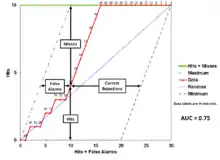
The TOC curve with four boxes indicates how a point on the TOC curve reveals the hits, misses, false alarms, and correct rejections. The TOC curve is an effective way to show the total information in the contingency table for all thresholds. The data used to create this TOC curve is available for download here. This dataset has 30 observations, each of which consists of values for a Boolean variable and an index variable. The observations are ranked from the greatest to the least value of the index. There are 31 thresholds, consisting of the 30 values of the index and one additional threshold that is greater than all the index values, which creates the point at the origin (0,0). Each point is labeled to indicate the value of each threshold. The horizontal axes ranges from 0 to 30 which is the number of observations in the dataset (P + Q). The vertical axis ranges from 0 to 10, which is the Boolean variable's number of presence observations P (i.e. hits + misses). TOC curves also show the threshold at which the diagnosed amount of presence matches the Boolean amount of presence, which is the threshold point that lies directly under the point where the maximum line meets the hits + misses line, as the TOC curve on the left illustrates. For a more detailed explanation of the construction of the TOC curve, please see Pontius Jr, Robert Gilmore; Si, Kangping (2014). "The total operating characteristic to measure diagnostic ability for multiple thresholds." International Journal of Geographical Information Science 28 (3): 570–583.”[1]
The following four pieces of information are the central entries in the contingency table for each threshold:
- The number of hits at each threshold is the distance between the threshold's point and the horizontal axis.
- The number of misses at each threshold is the distance between the threshold's point and the hits + misses horizontal line across the top of the graph.
- The number of false alarms at each threshold is the distance between threshold's point and the blue dashed Maximum line that bounds the left side of the TOC space.
- The number of correct rejections at each threshold is the distance between the threshold's point and the purple dashed Minimum line that bounds the right side of the TOC space.
TOC vs. ROC curves


These figures are the TOC and ROC curves using the same data and thresholds. Consider the point that corresponds to a threshold of 74. The TOC curve shows the number of hits, which is 3, and hence the number of misses, which is 7. Additionally, the TOC curve shows that the number of false alarms is 4 and the number of correct rejections is 16. At any given point in the ROC curve, it is possible to glean values for the ratios of false alarms/(false alarms+correct rejections) and hits/(hits+misses). For example, at threshold 74, it is evident that the x coordinate is 0.2 and the y coordinate is 0.3. However, these two values are insufficient to construct all entries of the underlying two-by-two contingency table.
Interpreting TOC curves
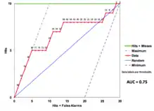
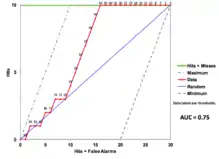
It is common to report the area under the curve (AUC) to summarize a TOC or ROC curve. However, condensing diagnostic ability into a single number fails to appreciate the shape of the curve. The following three TOC curves are TOC curves that have an AUC of 0.75 but have different shapes.

This TOC curve on the left exemplifies an instance in which the index variable has a high diagnostic ability at high thresholds near the origin, but random diagnostic ability at low thresholds near the upper right of the curve. The curve shows accurate diagnosis of presence until the curve reaches a threshold of 86. The curve then levels off and predicts around the random line.

This TOC curve exemplifies an instance in which the index variable has a medium diagnostic ability at all thresholds. The curve is consistently above the random line.

This TOC curve exemplifies an instance in which the index variable has random diagnostic ability at high thresholds and high diagnostic ability at low thresholds. The curve follows the random line at the highest thresholds near the origin, then the index variable diagnoses absence correctly as thresholds decrease near the upper right corner.
Area under the curve
When measuring diagnostic ability, a commonly reported measure is the area under the curve (AUC). The AUC is calculable from the TOC and the ROC. The value of the AUC is consistent for the same data whether you are calculating the area under the curve for a TOC curve or a ROC curve. The AUC indicates the probability that the diagnosis ranks a randomly chosen observation of Boolean presence higher than a randomly chosen observation of Boolean absence.[3] The AUC is appealing to many researchers because AUC summarizes diagnostic ability in a single number, however, the AUC has come under critique as a potentially misleading measure, especially for spatially explicit analyses.[3][4] Some features of the AUC that draw criticism include the fact that 1) AUC ignores the thresholds; 2) AUC summarizes the test performance over regions of the TOC or ROC space in which one would rarely operate; 3) AUC weighs omission and commission errors equally; 4) AUC does not give information about the spatial distribution of model errors; and, 5) the selection of spatial extent highly influences the rate of accurately diagnosed absences and the AUC scores.[5] However, most of those criticisms apply to many other metrics.
When using normalized units, the area under the curve (often referred to as simply the AUC) is equal to the probability that a classifier will rank a randomly chosen positive instance higher than a randomly chosen negative one (assuming 'positive' ranks higher than 'negative').[6] This can be seen as follows: the area under the curve is given by (the integral boundaries are reversed as large T has a lower value on the x-axis)
where is the score for a positive instance and is the score for a negative instance, and and are probability densities as defined in previous section.
It can further be shown that the AUC is closely related to the Mann–Whitney U,[7][8] which tests whether positives are ranked higher than negatives. It is also equivalent to the Wilcoxon test of ranks.[8] The AUC is related to the Gini coefficient () by the formula , where:
In this way, it is possible to calculate the AUC by using an average of a number of trapezoidal approximations.
It is also common to calculate the area under the TOC convex hull (ROC AUCH = ROCH AUC) as any point on the line segment between two prediction results can be achieved by randomly using one or the other system with probabilities proportional to the relative length of the opposite component of the segment.[10] It is also possible to invert concavities – just as in the figure the worse solution can be reflected to become a better solution; concavities can be reflected in any line segment, but this more extreme form of fusion is much more likely to overfit the data.[11]
Another problem with TOC AUC is that reducing the TOC Curve to a single number ignores the fact that it is about the tradeoffs between the different systems or performance points plotted and not the performance of an individual system, as well as ignoring the possibility of concavity repair, so that related alternative measures such as Informedness or DeltaP are recommended.[12][13] These measures are essentially equivalent to the Gini for a single prediction point with DeltaP' = informedness = 2AUC-1, whilst DeltaP = markedness represents the dual (viz. predicting the prediction from the real class) and their geometric mean is the Matthews correlation coefficient.
Whereas TOC AUC varies between 0 and 1 — with an uninformative classifier yielding 0.5 — the alternative measures known as informedness, Certainty [12] and Gini coefficient (in the single parameterization or single system case) all have the advantage that 0 represents chance performance whilst 1 represents perfect performance, and −1 represents the "perverse" case of full informedness always giving the wrong response.[14] Bringing chance performance to 0 allows these alternative scales to be interpreted as Kappa statistics. Informedness has been shown to have desirable characteristics for machine learning versus other common definitions of Kappa such as Cohen kappa and Fleiss kappa.[15]
Sometimes it can be more useful to look at a specific region of the TOC curve rather than at the whole curve. It is possible to compute partial AUC.[16] For example, one could focus on the region of the curve with low false positive rate, which is often of prime interest for population screening tests.[17] Another common approach for classification problems in which P ≪ N (common in bioinformatics applications) is to use a logarithmic scale for the x-axis.[18]
See also
References
- Pontius, Robert Gilmore; Si, Kangping (2014). "The total operating characteristic to measure diagnostic ability for multiple thresholds". International Journal of Geographical Information Science. 28 (3): 570–583. doi:10.1080/13658816.2013.862623. S2CID 29204880.
- Pontius, Robert Gilmore; Parmentier, Benoit (2014). "Recommendations for using the Relative Operating Characteristic (ROC)". Landscape Ecology. 29 (3): 367–382. doi:10.1007/s10980-013-9984-8. S2CID 254740981.
- Halligan, Steve; Altman, Douglas G.; Mallett, Susan (2015). "Disadvantages of using the area under the receiver operating characteristic curve to assess imaging tests: A discussion and proposal for an alternative approach". European Radiology. 25 (4): 932–939. doi:10.1007/s00330-014-3487-0. PMC 4356897. PMID 25599932.
- Powers, David Martin Ward (2012). "The problem of Area Under the Curve". 2012 IEEE International Conference on Information Science and Technology. pp. 567–573. doi:10.1109/ICIST.2012.6221710. ISBN 978-1-4577-0345-4. S2CID 11072457.
- Lobo, Jorge M.; Jiménez-Valverde, Alberto; Real, Raimundo (2008). "AUC: a misleading measure of the performance of predictive distribution models". Global Ecology and Biogeography. 17 (2): 145–151. doi:10.1111/j.1466-8238.2007.00358.x.
- Fawcett, Tom (2006); An introduction to ROC analysis, Pattern Recognition Letters, 27, 861–874.
- Hanley, James A.; McNeil, Barbara J. (1982). "The Meaning and Use of the Area under a Receiver Operating Characteristic (ROC) Curve". Radiology. 143 (1): 29–36. doi:10.1148/radiology.143.1.7063747. PMID 7063747. S2CID 10511727.
- Mason, Simon J.; Graham, Nicholas E. (2002). "Areas beneath the relative operating characteristics (ROC) and relative operating levels (ROL) curves: Statistical significance and interpretation" (PDF). Quarterly Journal of the Royal Meteorological Society. 128 (584): 2145–2166. Bibcode:2002QJRMS.128.2145M. CiteSeerX 10.1.1.458.8392. doi:10.1256/003590002320603584. S2CID 121841664. Archived from the original (PDF) on 2008-11-20.
- Hand, David J.; and Till, Robert J. (2001); A simple generalization of the area under the ROC curve for multiple class classification problems, Machine Learning, 45, 171–186.
- Provost, F.; Fawcett, T. (2001). "Robust classification for imprecise environments". Machine Learning. 42 (3): 203–231. arXiv:cs/0009007. doi:10.1023/a:1007601015854. S2CID 5415722.
- Flach, P.A.; Wu, S. (2005). "Repairing concavities in ROC curves." (PDF). 19th International Joint Conference on Artificial Intelligence (IJCAI'05). pp. 702–707.
- Powers, David MW (2012). "ROC-ConCert: ROC-Based Measurement of Consistency and Certainty" (PDF). Spring Congress on Engineering and Technology (SCET). Vol. 2. IEEE. pp. 238–241.
- Powers, David M.W. (2012). "The Problem of Area Under the Curve". International Conference on Information Science and Technology.
- Powers, David M. W. (2003). "Recall and Precision versus the Bookmaker" (PDF). Proceedings of the International Conference on Cognitive Science (ICSC-2003), Sydney Australia, 2003, pp. 529–534.
- Powers, David M. W. (2012). "The Problem with Kappa" (PDF). Conference of the European Chapter of the Association for Computational Linguistics (EACL2012) Joint ROBUS-UNSUP Workshop. Archived from the original (PDF) on 2016-05-18. Retrieved 2012-07-20.
- McClish, Donna Katzman (1989-08-01). "Analyzing a Portion of the ROC Curve". Medical Decision Making. 9 (3): 190–195. doi:10.1177/0272989X8900900307. PMID 2668680. S2CID 24442201.
- Dodd, Lori E.; Pepe, Margaret S. (2003). "Partial AUC Estimation and Regression". Biometrics. 59 (3): 614–623. doi:10.1111/1541-0420.00071. PMID 14601762. S2CID 23054670.
- Karplus, Kevin (2011); Better than Chance: the importance of null models, University of California, Santa Cruz, in Proceedings of the First International Workshop on Pattern Recognition in Proteomics, Structural Biology and Bioinformatics (PR PS BB 2011)
Further reading
- Pontius Jr, Robert Gilmore; Si, Kangping (2014). "The total operating characteristic to measure diagnostic ability for multiple thresholds". International Journal of Geographical Information Science. 28 (3): 570–583. doi:10.1080/13658816.2013.862623. S2CID 29204880.
- Pontius Jr, Robert Gilmore; Parmentier, Benoit (2014). "Recommendations for using the Relative Operating Characteristic (ROC)". Landscape Ecology. 29 (3): 367–382. doi:10.1007/s10980-013-9984-8. S2CID 254740981.
- Mas, Jean-François; Filho, Britaldo Soares; Pontius Jr, Robert Gilmore; Gutiérrez, Michelle Farfán; Rodrigues, Hermann (2013). "A suite of tools for ROC analysis of spatial models". ISPRS International Journal of Geo-Information. 2 (3): 869–887. Bibcode:2013IJGI....2..869M. doi:10.3390/ijgi2030869.
- Pontius Jr, Robert Gilmore; Pacheco, Pablo (2004). "Calibration and validation of a model of forest disturbance in the Western Ghats, India 1920–1990". GeoJournal. 61 (4): 325–334. doi:10.1007/s10708-004-5049-5. S2CID 155073463.
- Pontius Jr, Robert Gilmore; Batchu, Kiran (2003). "Using the relative operating characteristic to quantify certainty in prediction of location of land cover change in India". Transactions in GIS. 7 (4): 467–484. doi:10.1111/1467-9671.00159. S2CID 14452746.
- Pontius Jr, Robert Gilmore; Schneider, Laura (2001). "Land-use change model validation by a ROC method for the Ipswich watershed, Massachusetts, USA". Agriculture, Ecosystems & Environment. 85 (1–3): 239–248. doi:10.1016/s0167-8809(01)00187-6.
External links
- An Introduction to the Total Operating Characteristic: Utility in Land Change Model Evaluation
- TOC utilization in Wildfire Risk
- How to run the TOC Package in R
- TOC R package on Github
- Excel Workbook for generating TOC curves
- Google Earth Engine TOC Curve Tutorial
- Google Earth Engine TOC Curve Source Code