Lesson 14: Creating More Complex Formulas

/en/excel2016/intro-to-formulas/content/

Introduction

You may have experience working with formulas that contain only one operator, such as 7+9. More complex formulas can contain several mathematical operators, such as 5+2*8. When there's more than one operation in a formula, the order of operations tells Excel which operation to calculate first. To write formulas that will give you the correct answer, you'll need to understand the order of operations.

Watch the video below to learn more about complex formulas.

The order of operations

Excel calculates formulas based on the following order of operations:

  1. Operations enclosed in parentheses
  2. Exponential calculations (3^2, for example)
  3. Multiplication and division, whichever comes first
  4. Addition and subtraction, whichever comes first

A mnemonic that can help you remember the order is PEMDAS, or Please Excuse My Dear Aunt Sally.

Click the arrows in the slideshow below to learn how the order of operations is used to calculate formulas in Excel.

  • PEMDAS, 10+(6-3)/2^2*4-1

    While this formula may look complicated, we can use the order of operations step by step to find the right answer.

  • P parentheses: 10+(6-3)/2^2*4-1

    First, we'll start by calculating anything inside parentheses. In this case, there's only one thing we need to calculate: 6-3=3.

  • E exponents: 10+3/2^2*4-1

    As you can see, the formula already looks simpler. Next, we'll look to see if there are any exponents. There is one: 2^2=4.

  • MD multiplication division, whichever comes first: 10+3/4*4-1

    Next, we'll solve any multiplication and division, working from left to right. Because the division operation comes before the multiplication, it's calculated first: 3/4=0.75.

  • MD multiplication division, whichever comes first: 10+0.75*4-1

    Now, we'll solve our remaining multiplication operation: 0.75*4=3.

  • AS addition subtraction, whichever comes first: 10+3-1

    Next, we'll calculate any addition or subtraction, again working from left to right. Addition comes first: 10+3=13.

  • AS addition subtraction, whichever comes first: 13-1

    Finally, we have one remaining subtraction operation: 13-1=12.

  • answer: 13-1=12

    Now we have our answer: 12. And this is the exact same result you would get if you entered the formula into Excel.

  • GCFLearnFree.org

Creating complex formulas

In the example below, we'll demonstrate how Excel uses the order of operations to solve a more complex formula. Here, we want to calculate the cost of sales tax for a catering invoice. To do this, we'll write our formula as =(D3+D4+D5)*0.075 in cell D6. This formula will add the prices of our items, then multiply that value by the 7.5% tax rate (which is written as 0.075) to calculate the answer.

Creating a complex formula

Excel follows the order of operations and first adds the values inside the parentheses: (45.80+68.70+159.60) = 274.10. It then multiplies that value by the tax rate: 274.10*0.075. The result will show that the sales tax is $20.56.

Formula result

It's especially important to follow the order of operations when creating a formula. Otherwise, Excel won't calculate the results accurately. In our example, if the parentheses are not included, the multiplication is calculated first and the result is incorrect. Parentheses are often the best way to define which calculations will be performed first in Excel.

Formula without parentheses

To create a complex formula using the order of operations:

In the example below, we'll use cell references along with numerical values to create a complex formula that will calculate the subtotal for a catering invoice. The formula will calculate the cost of each menu item first, then add these values.

  1. Select the cell that will contain the formula. In our example, we'll select cell C5.
    Selecting a cell
  2. Enter your formula. In our example, we'll type =B3*C3+B4*C4. This formula will follow the order of operations, first performing the multiplication: 2.79*35 = 97.65 and 2.29*20 = 45.80. It then will add these values to calculate the total: 97.65+45.80.
    Creating a complex formula
  3. Double-check your formula for accuracy, then press Enter on your keyboard. The formula will calculate and display the result. In our example, the result shows that the subtotal for the order is $143.45.
    Formula result

You can add parentheses to any equation to make it easier to read. While it won't change the result of the formula in this example, we could enclose the multiplication operations within parentheses to clarify that they will be calculated before the addition.

Formula with parentheses

Excel will not always tell you if your formula contains an error, so it's up to you to check all of your formulas. To learn how to do this, you can read the Double-Check Your Formulas lesson from our Excel Formulas tutorial.

Challenge!

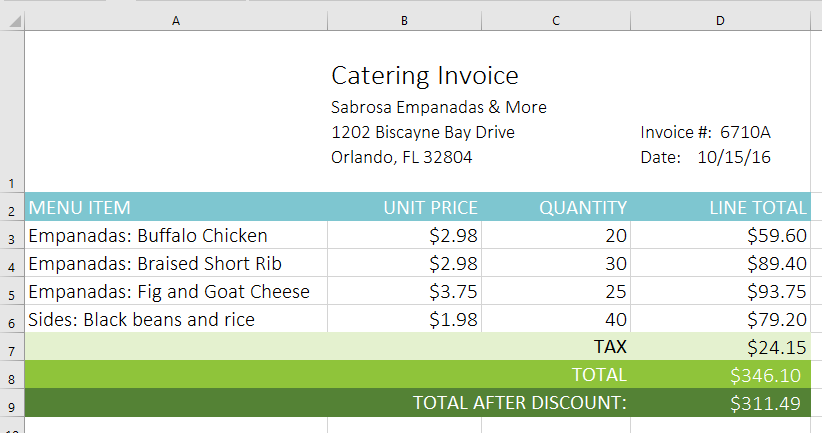
For this challenge, you are going to work with another invoice like the one in our example. In the invoice, you will find the amount of tax for the order, the order's total, and the order's total if you were given a 10% discount.
  1. Open our practice workbook.
  2. Click the Challenge worksheet tab in the bottom-left of the workbook.
  3. In cell D7, create a formula that calculates the tax for the invoice. Use a sales tax rate of 7.5%.
  4. In cell D8, create a formula that finds the total for the order. In other words, this formula should add cells D3:D7.
  5. In cell D9 create a formula that calculates the total after a 10% discount. If you need help understanding how to take a percentage off of a total, check out our lesson on Discounts, Markdowns, and Sales.
  6. When you're finished, your spreadsheet should look like this:
    Complex Formulas Challenge

/en/excel2016/relative-and-absolute-cell-references/content/