

/en/excel2016/page-layout-and-printing/content/
One of the most powerful features in Excel is the ability to calculate numerical information using formulas. Just like a calculator, Excel can add, subtract, multiply, and divide. In this lesson, we'll show you how to use cell references to create simple formulas.
Watch the video below to learn more about creating formulas in Excel.
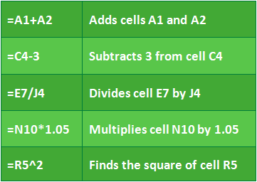
Excel uses standard operators for formulas, such as a plus sign for addition (+), a minus sign for subtraction (-), an asterisk for multiplication (*), a forward slash for division (/), and a caret (^) for exponents.

All formulas in Excel must begin with an equals sign (=). This is because the cell contains, or is equal to, the formula and the value it calculates.
While you can create simple formulas in Excel using numbers (for example, =2+2 or =5*5), most of the time you will use cell addresses to create a formula. This is known as making a cell reference. Using cell references will ensure that your formulas are always accurate because you can change the value of referenced cells without having to rewrite the formula.
In the formula below, cell A3 adds the values of cells A1 and A2 by making cell references:
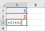
When you press Enter, the formula calculates and displays the answer in cell A3:

If the values in the referenced cells change, the formula automatically recalculates:

By combining a mathematical operator with cell references, you can create a variety of simple formulas in Excel. Formulas can also include a combination of cell references and numbers, as in the examples below:
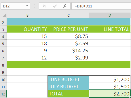
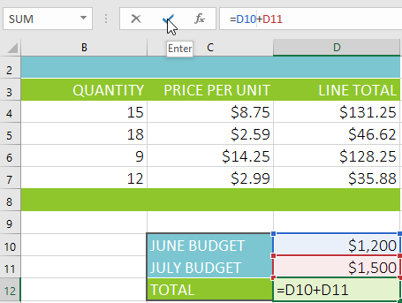
In our example below, we'll use a simple formula and cell references to calculate a budget.
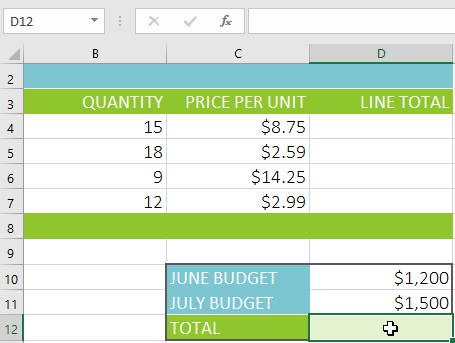

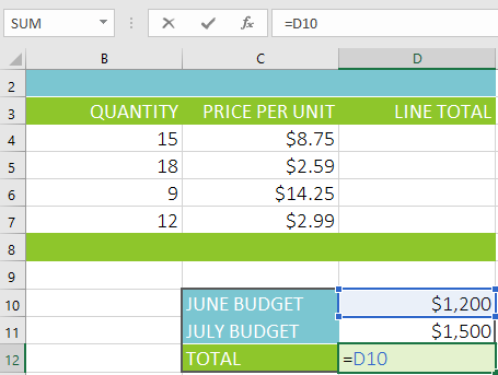

If the result of a formula is too large to be displayed in a cell, it may appear as pound signs (#######) instead of a value. This means the column is not wide enough to display the cell content. Simply increase the column width to show the cell content.
The true advantage of cell references is that they allow you to update data in your worksheet without having to rewrite formulas. In the example below, we've modified the value of cell D10 from $1,200 to $1,800. The formula in D12 will automatically recalculate and display the new value in cell D12.

Excel will not always tell you if your formula contains an error, so it's up to you to check all of your formulas. To learn how to do this, you can read the Double-Check Your Formulas lesson from our Excel Formulas tutorial.
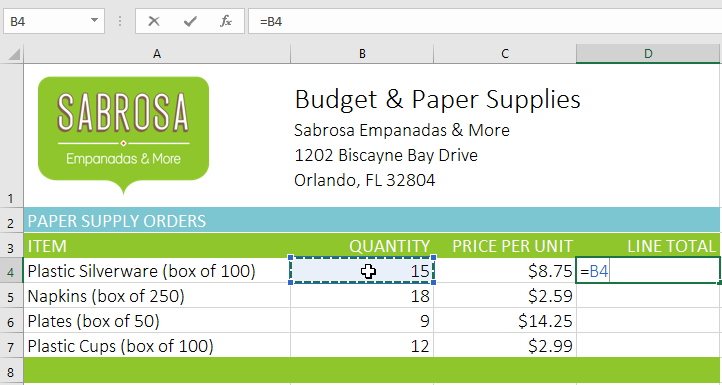
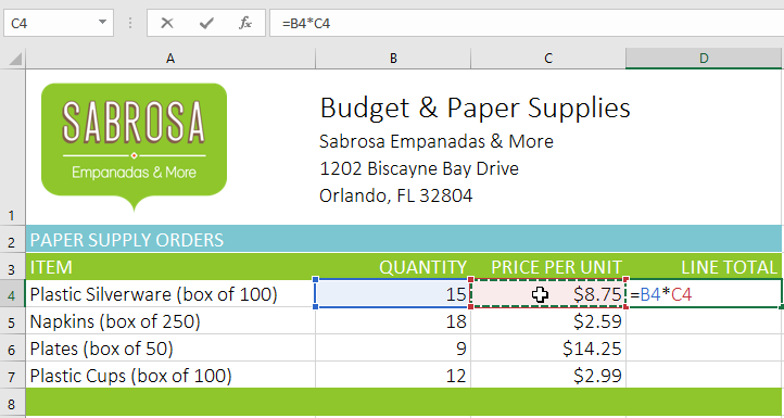
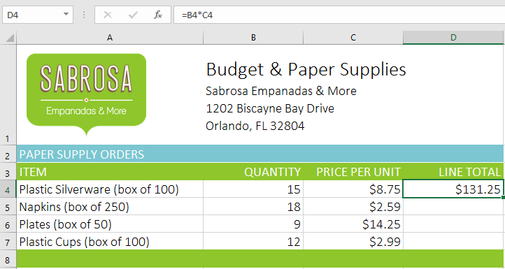
Instead of typing cell addresses manually, you can point and click the cells you want to include in your formula. This method can save a lot of time and effort when creating formulas. In our example below, we'll create a formula to calculate the cost of ordering several boxes of plastic silverware.

Formulas can also be copied to adjacent cells with the fill handle, which can save a lot of time and effort if you need to perform the same calculation multiple times in a worksheet. The fill handle is the small square at the bottom-right corner of the selected cell(s).
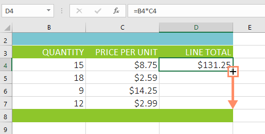
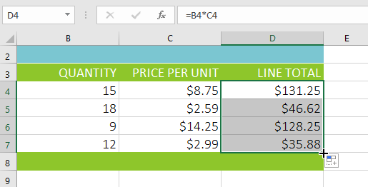
Sometimes you may want to modify an existing formula. In the example below, we've entered an incorrect cell address in our formula, so we'll need to correct it.

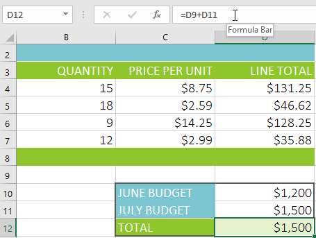
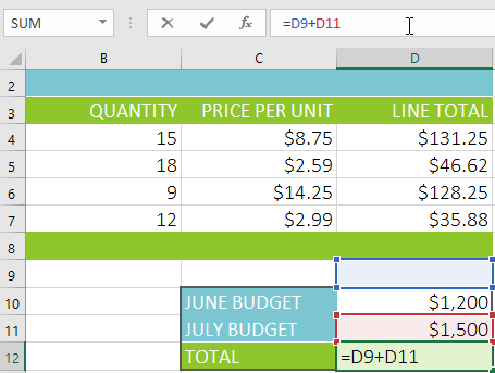

If you change your mind, you can press the Esc key on your keyboard or click the Cancel command in the formula bar to avoid accidentally making changes to your formula.

To show all of the formulas in a spreadsheet, you can hold the Ctrl key and press ` (grave accent). The grave accent key is usually located in the top-left corner of the keyboard. You can press Ctrl+` again to switch back to the normal view.

/en/excel2016/creating-more-complex-formulas/content/