Cox–Ingersoll–Ross model
In mathematical finance, the Cox–Ingersoll–Ross (CIR) model describes the evolution of interest rates. It is a type of "one factor model" (short-rate model) as it describes interest rate movements as driven by only one source of market risk. The model can be used in the valuation of interest rate derivatives. It was introduced in 1985[1] by John C. Cox, Jonathan E. Ingersoll and Stephen A. Ross as an extension of the Vasicek model.

The model

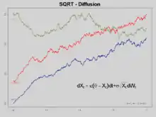
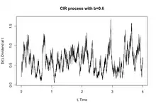
The CIR model specifies that the instantaneous interest rate follows the stochastic differential equation, also named the CIR Process:
where is a Wiener process (modelling the random market risk factor) and , , and are the parameters. The parameter corresponds to the speed of adjustment to the mean , and to volatility. The drift factor, , is exactly the same as in the Vasicek model. It ensures mean reversion of the interest rate towards the long run value , with speed of adjustment governed by the strictly positive parameter .
The standard deviation factor, , avoids the possibility of negative interest rates for all positive values of and . An interest rate of zero is also precluded if the condition
is met. More generally, when the rate () is close to zero, the standard deviation () also becomes very small, which dampens the effect of the random shock on the rate. Consequently, when the rate gets close to zero, its evolution becomes dominated by the drift factor, which pushes the rate upwards (towards equilibrium).
This process can be defined as a sum of squared Ornstein–Uhlenbeck process. The CIR is an ergodic process, and possesses a stationary distribution. The same process is used in the Heston model to model stochastic volatility.
Distribution
- Future distribution
- The distribution of future values of a CIR process can be computed in closed form:
- where , and Y is a non-central chi-squared distribution with degrees of freedom and non-centrality parameter . Formally the probability density function is:
- where , , , and is a modified Bessel function of the first kind of order .
- Asymptotic distribution
- Due to mean reversion, as time becomes large, the distribution of will approach a gamma distribution with the probability density of:
- where and .
Derivation of asymptotic distribution |
|---|
|
To derive the asymptotic distribution for the CIR model, we must use the Fokker-Planck equation: Our interest is in the particular case when , which leads to the simplified equation: Defining and and rearranging terms leads to the equation: Integrating shows us that: Over the range , this density describes a gamma distribution. Therefore, the asymptotic distribution of the CIR model is a gamma distribution. |
Properties
- Mean reversion,
- Level dependent volatility (),
- For given positive the process will never touch zero, if ; otherwise it can occasionally touch the zero point,
- , so long term mean is ,
Calibration
- The continuous SDE can be discretized as follows
- which is equivalent to
- provided is n.i.i.d. (0,1). This equation can be used for a linear regression.
- Martingale estimation
- Maximum likelihood
Simulation
Stochastic simulation of the CIR process can be achieved using two variants:
- Discretization
- Exact
Bond pricing
Under the no-arbitrage assumption, a bond may be priced using this interest rate process. The bond price is exponential affine in the interest rate:
where
Extensions
A CIR process is a special case of a basic affine jump diffusion, which still permits a closed-form expression for bond prices. Time varying functions replacing coefficients can be introduced in the model in order to make it consistent with a pre-assigned term structure of interest rates and possibly volatilities. The most general approach is in Maghsoodi (1996).[2] A more tractable approach is in Brigo and Mercurio (2001b)[3] where an external time-dependent shift is added to the model for consistency with an input term structure of rates.
A significant extension of the CIR model to the case of stochastic mean and stochastic volatility is given by Lin Chen (1996) and is known as Chen model. A more recent extension for handling cluster volatility, negative interest rates and different distributions is the so-called "CIR #" by Orlando, Mininni and Bufalo (2018,[4] 2019,[5][6] 2020,[7] 2021,[8] 2023[9]) and a simpler extension focussing on negative interest rates was proposed by Di Francesco and Kamm (2021,[10] 2022[11]), which are referred to as the CIR- and CIR-- models.
See also
References
- "A Theory of the Term Structure of Interest Rates - The Econometric Society". www.econometricsociety.org. Retrieved 2023-10-14.
- Maghsoodi, Yoosef (January 1996). "SOLUTION OF THE EXTENDED CIR TERM STRUCTURE AND BOND OPTION VALUATION". Mathematical Finance. 6 (1): 89–109. doi:10.1111/j.1467-9965.1996.tb00113.x. ISSN 0960-1627.
- Brigo, Damiano; Mercurio, Fabio (2001-07-01). "A deterministic–shift extension of analytically–tractable and time–homogeneous short–rate models". Finance and Stochastics. 5 (3): 369–387. doi:10.1007/PL00013541. ISSN 0949-2984.
- Orlando, Giuseppe; Mininni, Rosa Maria; Bufalo, Michele (2018). "A New Approach to CIR Short-Term Rates Modelling". New Methods in Fixed Income Modeling. Contributions to Management Science. Springer International Publishing: 35–43. doi:10.1007/978-3-319-95285-7_2. ISBN 978-3-319-95284-0.
- Orlando, Giuseppe; Mininni, Rosa Maria; Bufalo, Michele (1 January 2019). "A new approach to forecast market interest rates through the CIR model". Studies in Economics and Finance. 37 (2): 267–292. doi:10.1108/SEF-03-2019-0116. ISSN 1086-7376. S2CID 204424299.
- Orlando, Giuseppe; Mininni, Rosa Maria; Bufalo, Michele (19 August 2019). "Interest rates calibration with a CIR model". The Journal of Risk Finance. 20 (4): 370–387. doi:10.1108/JRF-05-2019-0080. ISSN 1526-5943. S2CID 204435499.
- Orlando, Giuseppe; Mininni, Rosa Maria; Bufalo, Michele (July 2020). "Forecasting interest rates through Vasicek and CIR models: A partitioning approach". Journal of Forecasting. 39 (4): 569–579. arXiv:1901.02246. doi:10.1002/for.2642. ISSN 0277-6693. S2CID 126507446.
- Orlando, Giuseppe; Bufalo, Michele (2021-05-26). "Interest rates forecasting: Between Hull and White and the CIR#—How to make a single‐factor model work". Journal of Forecasting. 40 (8): 1566–1580. doi:10.1002/for.2783. ISSN 0277-6693.
- Orlando, Giuseppe; Bufalo, Michele (2023-07-14). "Time series forecasting with the CIR# model: from hectic markets sentiments to regular seasonal tourism". Technological and Economic Development of Economy. 29 (4): 1216–1238. doi:10.3846/tede.2023.19294. ISSN 2029-4921.
- Di Francesco, Marco; Kamm, Kevin (4 October 2021). "How to handle negative interest rates in a CIR framework". SeMa Journal. 79 (4): 593–618. doi:10.1007/s40324-021-00267-w. S2CID 235358123.
- Di Francesco, Marco; Kamm, Kevin (2022). "On the Deterministic-Shift Extended CIR Model in a Negative Interest Rate Framework". International Journal of Financial Studies. 10 (2): 38. doi:10.3390/ijfs10020038.
Further References
- Hull, John C. (2003). Options, Futures and Other Derivatives. Upper Saddle River, NJ: Prentice Hall. ISBN 0-13-009056-5.
- Cox, J.C., J.E. Ingersoll and S.A. Ross (1985). "A Theory of the Term Structure of Interest Rates". Econometrica. 53 (2): 385–407. doi:10.2307/1911242. JSTOR 1911242.
{{cite journal}}: CS1 maint: multiple names: authors list (link) - Maghsoodi, Y. (1996). "Solution of the extended CIR Term Structure and Bond Option Valuation". Mathematical Finance. 6 (6): 89–109. doi:10.1111/j.1467-9965.1996.tb00113.x.
- Damiano Brigo; Fabio Mercurio (2001). Interest Rate Models — Theory and Practice with Smile, Inflation and Credit (2nd ed. 2006 ed.). Springer Verlag. ISBN 978-3-540-22149-4.
- Brigo, Damiano; Fabio Mercurio (2001b). "A deterministic-shift extension of analytically tractable and time-homogeneous short rate models". Finance & Stochastics. 5 (3): 369–388. doi:10.1007/PL00013541. S2CID 35316609.
- Open Source library implementing the CIR process in python
- Orlando, Giuseppe; Mininni, Rosa Maria; Bufalo, Michele (2020). "Forecasting interest rates through Vasicek and CIR models: A partitioning approach". Journal of Forecasting. 39 (4): 569–579. arXiv:1901.02246. doi:10.1002/for.2642. ISSN 1099-131X. S2CID 126507446.