wikiHow is a “wiki,” similar to Wikipedia, which means that many of our articles are co-written by multiple authors. To create this article, volunteer authors worked to edit and improve it over time.
This article has been viewed 14,092 times.
Learn more...
Maxwell's celebrated equations, along with the Lorentz force law, describe electrodynamics in a highly succinct fashion. However, what appears to be four elegant equations are actually eight partial differential equations that are difficult to solve for, given charge density and current density since Faraday's Law and the Ampere-Maxwell Law are vector equations with three components each. Reformulating Maxwell's equations in terms of vector and scalar potentials makes solving for the electric field and the magnetic field much easier. In quantum electrodynamics, equations are formulated almost exclusively in terms of the potentials rather than the fields themselves. We'll show you how to write Maxwell's equations in potential form and go over gauge transformations to simplify the equations.


Steps
Rewriting in Terms of Potentials
-
1Begin with Maxwell's equations. Below, and are the electric and magnetic constants, respectively (we are working in SI units).
-
2Define the magnetic potential. From Gauss' Law of Magnetism, we see that magnetic fields are divergenceless via In vector calculus, a theorem is that the divergence of a curl is always zero. Therefore, we can rewrite in terms of a magnetic potential
- From here, we see that magnetic potential is a vector potential. This definition automatically satisfies Gauss' Law of Magnetism through the aforementioned vector identity
Advertisement -
3Rewrite Faraday's Law in terms of the magnetic potential. Recall back in electrostatics that was a conservative field (i.e. ), which allowed us to write it in terms of a scalar potential In electrodynamics, is no longer conservative, due to the presence of a changing field induced by moving charged particles. However, substituting into Faraday's Law returns an equation which we can take the scalar gradient of. By doing so, our potential definition automatically satisfies another of Maxwell's equations.
- Now, we can write the quantity in parentheses in terms of a scalar potential.
- Solve for to obtain the electric field in terms of potentials.
-
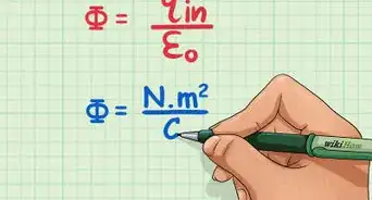
4Rewrite Gauss' Law in terms of potentials. Now that we are done with the two homogeneous equations, we can work our way with the other two.
-
5Rewrite the Ampere-Maxwell Law in terms of potentials.
- Make use of the BAC-CAB identity. For the vector calculus form, it reads as
- Rearrange so that the Laplacian and the gradient terms are together.
- Through rewriting Gauss' Law and the Ampere-Maxwell Law in terms of potentials, we have reduced Maxwell's equations from four equations to two. Furthermore, we have reduced the number of components to just four - the scalar potential and the three components of the vector potential.
- However, no one ever encounters Maxwell's equations written like this.


Gauge Transformations
-
1Revisit the definitions of the scalar and vector potentials. It turns out that and are not uniquely defined, since an appropriate change in these quantities results in the same and fields. These changes in the potentials are called gauge transformations. In this section, we outline two of the most common gauge transformations that greatly simplify Maxwell's equations.
-
2Account for gauge freedom. Let's label the changes as and
- If the vector potentials give the same then Then, we can write in terms of a scalar
- Similarly, if both potentials give the same then
- Solving for by integrating both sides adds a constant that depends on time. However, this constant does not affect the gradient of so we can neglect it.
-
3Rewrite the gauge freedoms in terms of . By manipulating these transformations in an appropriate manner, we can change the divergence of to simplify Maxwell's equations by choosing a that satisfies the conditions we want.
-
4Obtain the Coulomb gauge. Set
- This is the Coulomb gauge, which reduces the scalar potential equation to Poisson's equation, but results in a rather complicated vector potential equation.
-
5Obtain the Lorenz gauge. Set
- This is the Lorenz gauge, which results in manifest Lorentz covariance. The two potential equations are now in the same form of the inhomogeneous wave equation.