Quick step-by-step guide to creating a new pivot table column
This article was co-authored by wikiHow staff writer, Kyle Smith. Kyle Smith is a wikiHow Technology Writer, learning and sharing information about the latest technology. He has presented his research at multiple engineering conferences and is the writer and editor of hundreds of online electronics repair guides. Kyle received a BS in Industrial Engineering from Cal Poly, San Luis Obispo.
The wikiHow Tech Team also followed the article's instructions and verified that they work.
This article has been viewed 587,089 times.
Learn more...
This wikiHow teaches you how to insert a new column into a pivot table in Microsoft Excel with the pivot table tools. You can easily change an existing row, field, or value to a column, or create a new calculated field column with a custom formula.
Things You Should Know
- Show the Field List by going to PivotTable Analyze > Field List.
- Drag field items to the Columns area in the Field List to create new columns.
- Go to PivotTable Analyze > Fields, Items, & Sets > Calculated Field to make a custom field.
Steps
Changing a Field to Column
-
1Open the Excel file with the pivot table you want to edit. Find and double-click your Excel file on your computer to open it.
- If you haven't made your pivot table yet, open a new Excel document and create a pivot table before continuing.
-
2Click any cell on the pivot table. This will select the table, and show the “PivotTable Analyze” and “Design” tabs on the toolbar ribbon at the top.Advertisement
-
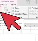
3Click the PivotTable Analyze tab at the top. You can find this tab alongside other tabs like Formulas, Insert, and View at the top of the app window. It will show your pivot table tools on the toolbar ribbon.[1]
- On some versions, this tab may just be named Analyze, and on others, you can find it as Options under the "Pivot Table Tools" heading.
-
4Click the Field List button on the toolbar ribbon. You can find this button on the right-hand side of the “PivotTable Analyze” tab. It will open a list of all the fields, rows, columns, and values in the selected table.
-
5Check the box next to any item on the “PivotTable Fields” list. This will calculate the summary of your original data in the selected category, and add it to your pivot table.
- Typically, non-numeric fields are added as rows, and numeric fields are added as values.
- You can uncheck the checkbox here anytime to remove the field from your pivot table.
-
6Drag and drop any field item to the "Columns" section. This will move the selected category to the Columns list, and re-design your pivot table with the newly added column.
- For example, if you have a column of years called “Years” in your source data, you can add the “Years” field to the Columns area to create columns for each year, showing values for each individual year.
- You can drag the field item name from the list of fields or from another area (Filters, Rows, Values).
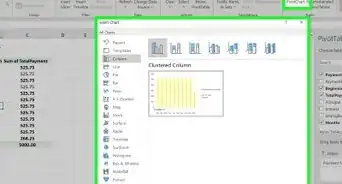
- Now you’re ready to analyze the data and make a few charts using the pivot table.


Adding a Calculated Field
-
1Open the Excel document you want to edit. Double-click the Excel document that contains your pivot table. This method will create a custom field using the existing fields and data.
- If you haven't yet made the pivot table, open a new Excel document and create a pivot table before continuing.
-
2Select the pivot table you want to edit. Click the pivot table on your worksheet to select and edit it.
-
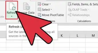
3Click the PivotTable Analyze tab. This tab is in the middle of the toolbar ribbon at the top of the Excel window. It will open your pivot table tools on the toolbar ribbon.
- On different versions, this tab may be named Analyze, or Options under the "Pivot Table Tools" heading.
-
4Click the Fields, Items, & Sets button on the toolbar ribbon. This button looks like an "fx" sign on a table icon on the far-right end of the toolbar. It will open a drop-down menu.
-
5Click Calculated Field on the drop-down menu. It will open a new window where you can add a new, custom column to your pivot table.
-
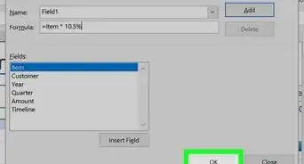
6Enter a name for your column in the "Name" field . Click the Name field, and type in the name you want to use for your new column. This name will appear at the top of the column.
-
7Enter a formula for your new column in the "Formula" field. Click the “Formula” field below “Name”, and type the formula you want to use for calculating your new column's data values.
- Make sure you type the formula on the right side of the "=" sign.
- Optionally, you can also select an existing column, and add it to your formula as a value:
- Select the field you want to add in the Fields section.
- Click Insert Field to add it to your formula.
- For example, if you have the fields “revenue” and “costs”, you could subtract them to get a “profit” calculated field.
-
8Click OK. Doing so will add the column to the right side of your pivot table.
- Alternatively, click Add to create the calculated field without closing the “Insert Calculated Field” window. This allows you to add additional calculated fields.
- You can reorder the columns by dragging the field items in the pivot table “Column” area.


Warnings
- Always remember to save your work when you're done.⧼thumbs_response⧽


References
About This Article

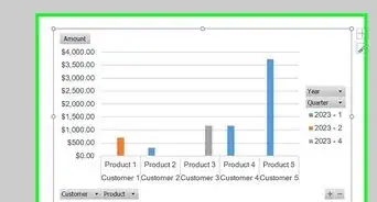
1. Click on the PivotTable.
2. Click the checkbox of the field you want to add.
3. Right-click on the added field.
4. Select Move to... Column Labels or Values.