X
wikiHow is a “wiki,” similar to Wikipedia, which means that many of our articles are co-written by multiple authors. To create this article, volunteer authors worked to edit and improve it over time.
This article has been viewed 103,787 times.
Learn more...
The matrix equation involves a matrix acting on a vector to produce another vector. In general, the way acts on is complicated, but there are certain cases where the action maps to the same vector, multiplied by a scalar factor.


Eigenvalues and eigenvectors have immense applications in the physical sciences, especially quantum mechanics, among other fields.
Steps
-
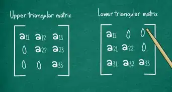
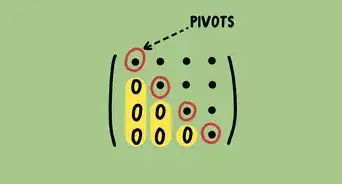
1Understand determinants. The determinant of a matrix when is non-invertible. When this occurs, the null space of becomes non-trivial - in other words, there are non-zero vectors that satisfy the homogeneous equation [1]
-
2Write out the eigenvalue equation. As mentioned in the introduction, the action of on is simple, and the result only differs by a multiplicative constant called the eigenvalue. Vectors that are associated with that eigenvalue are called eigenvectors.[2]
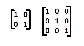
- We can set the equation to zero, and obtain the homogeneous equation. Below, is the identity matrix.
Advertisement -
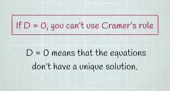
3Set up the characteristic equation. In order for to have non-trivial solutions, the null space of must be non-trivial as well.
- The only way this can happen is if This is the characteristic equation.
-
4Obtain the characteristic polynomial. yields a polynomial of degree for matrices.
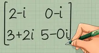
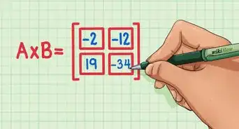
- Consider the matrix
- Notice that the polynomial seems backwards - the quantities in parentheses should be variable minus number, rather than the other way around. This is easy to deal with by moving the 12 to the right and multiplying by to both sides to reverse the order.
-
5Solve the characteristic polynomial for the eigenvalues. This is, in general, a difficult step for finding eigenvalues, as there exists no general solution for quintic functions or higher polynomials. However, we are dealing with a matrix of dimension 2, so the quadratic is easily solved.
-
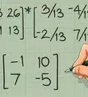
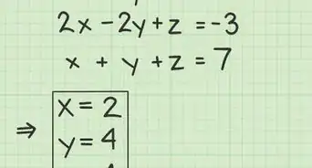
6Substitute the eigenvalues into the eigenvalue equation, one by one. Let's substitute first.[3]
- The resulting matrix is obviously linearly dependent. We are on the right track here.
-
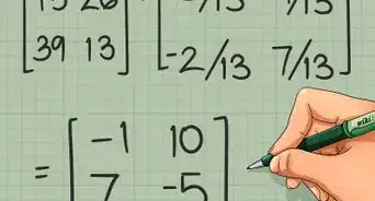
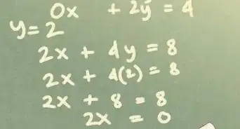
7Row-reduce the resulting matrix. With larger matrices, it may not be so obvious that the matrix is linearly dependent, and so we must row-reduce. Here, however, we can immediately perform the row operation to obtain a row of 0's.[4]
- The matrix above says that Simplify and reparameterize as it is a free variable.
-
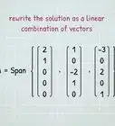
8Obtain the basis for the eigenspace. The previous step has led us to the basis of the null space of - in other words, the eigenspace of with eigenvalue 5.
- Performing steps 6 to 8 with results in the following eigenvector associated with eigenvalue -2.
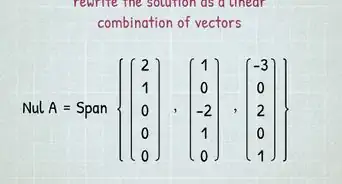
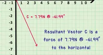
- These are the eigenvectors associated with their respective eigenvalues. For the basis of the entire eigenspace of we write


Advertisement
Community Q&A
-
QuestionWhy do we replace y with 1 and not any other number while finding eigenvectors?
 Community AnswerFor simplicity. Eigenvectors are only defined up to a multiplicative constant, so the choice to set the constant equal to 1 is often the simplest.
 -
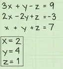
QuestionHow do you find the eigenvectors of a 3x3 matrix?
 AlphabetCommunity AnswerFirst, find the solutions x for det(A - xI) = 0, where I is the identity matrix and x is a variable. The solutions x are your eigenvalues. Let's say that a, b, c are your eignevalues. Now solve the systems [A - aI | 0], [A - bI | 0], [A - cI | 0]. The basis of the solution sets of these systems are the eigenvectors.
Advertisement

References
- ↑ www.math.lsa.umich.edu/~kesmith/ProofDeterminantTheorem.pdf
- ↑ http://tutorial.math.lamar.edu/Classes/DE/LA_Eigen.aspx
- ↑ https://www.intmath.com/matrices-determinants/7-eigenvalues-eigenvectors.php
- ↑ https://www.mathportal.org/algebra/solving-system-of-linear-equations/row-reduction-method.php
- ↑ http://www.math.lsa.umich.edu/~hochster/419/det.html
About This Article
Advertisement