How to Solve the Series RLC Circuit

Last Updated: July 14, 2018

The series RLC circuit is a circuit that contains a resistor, inductor, and a capacitor hooked up in series. The governing differential equation of this system is very similar to that of a damped harmonic oscillator encountered in classical mechanics.

Part 1

Part 1 of 3:

No Voltage Source

1
Use Kirchhoff's voltage law to relate the components of the circuit. Kirchhoff's voltage law for a series RLC circuit says that $V_{R}+V_{L}+V_{C}=V(t),$ $V_{{R}}+V_{{L}}+V_{{C}}=V(t),$ where $V(t)$ $V(t)$ is the time-dependent voltage source. In this section, we investigate the case without this source to obtain the solution to a homogeneous equation. We then tackle the slightly more complicated task of finding the steady-state solution. The diagram above shows an example of an RLC circuit.
- Electric current $I$ is related to charge by the relation $I={\dot {Q}},$ where $Q$ is electric charge and the dot signifies a time derivative.
- Ohm's law says that the voltage across a resistor is linearly proportional to the current: $V_{R}=IR.$ This can be written as $V_{R}=R{\dot {Q}}.$
- The voltage across an inductor is given by $V_{I}=L{\dot {I}},$ where $L$ is the inductance. As before, we can write this as $V_{I}=L{\ddot {Q}}.$
- The voltage across a capacitor is given by the relation $V_{C}={\frac {1}{C}}Q.$
- The governing differential equation is then given below.
  - $L{\ddot {Q}}+R{\dot {Q}}+{\frac {1}{C}}Q=0$
2
Relate the coefficients to the standard form of the harmonic oscillator equation.
- This more applicable form of the equation is given below. We can see from inspection that $\omega _{0}^{2}={\frac {1}{LC}}$ $\omega _{{0}}^{{2}}={\frac {1}{LC}}$ and $\beta ={\frac {R}{2L}}.$ $\beta ={\frac {R}{2L}}.$ $\omega _{0}$ $\omega _{{0}}$ refers to the frequency of the system, while $\beta$ $\beta$ is a parameter, also in units of angular frequency, that simplifies calculations. This parameter is called the attenuation and measures how quickly the transient response of the circuit dies away. We can apply this equation to the classical harmonic oscillator as well, or any system whose behavior is predominantly oscillatory in nature.
  - ${\ddot {Q}}+2\beta {\dot {Q}}+\omega _{0}^{2}Q=0$
Advertisement
3
Solve the characteristic equation to find the complementary solution.
- The solutions to the characteristic equation are very simple, and we can see why we deal with this equation instead.
  - $r^{2}+2\beta r+\omega _{0}^{2}=0$
  - $r=-\beta \pm {\sqrt {\beta ^{2}-\omega _{0}^{2}}}$
- We know that physically, the capacitance is usually a very small quantity. Capacitors are usually measured in nanofarads or microfarads, whereas resistors can be on the order of ohms to megaohms. It is therefore not unreasonable to suggest that $\omega _{0}^{2}>\beta ^{2}$ $\omega _{{0}}^{{2}}>\beta ^{{2}}$ so that the square root is negative and the solutions are oscillatory rather than exponential in nature. From the theory of differential equations, we obtain the complementary solution, where we write $\omega _{d}={\sqrt {\omega _{0}^{2}-\beta ^{2}}}$ $\omega _{{d}}={\sqrt {\omega _{{0}}^{{2}}-\beta ^{{2}}}}$ as the damped frequency.
  - $Q_{c}(t)=e^{-\beta t}\left(c_{1}\cos \omega _{d}t+c_{2}\sin \omega _{d}t\right)$
4
Rewrite the solution in the form with a phase factor. We can convert this solution into a slightly more familiar form by performing the following manipulation.
- Multiply the solution by ${\frac {\sqrt {c_{1}^{2}+c_{2}^{2}}}{\sqrt {c_{1}^{2}+c_{2}^{2}}}}.$ ${\frac {{\sqrt {c_{{1}}^{{2}}+c_{{2}}^{{2}}}}}{{\sqrt {c_{{1}}^{{2}}+c_{{2}}^{{2}}}}}}.$
  - $e^{-\beta t}{\sqrt {c_{1}^{2}+c_{2}^{2}}}\left({\frac {c_{1}}{\sqrt {c_{1}^{2}+c_{2}^{2}}}}\cos \omega _{d}t+{\frac {c_{2}}{\sqrt {c_{1}^{2}+c_{2}^{2}}}}\sin \omega _{d}t\right)$
- Draw a right triangle with angle $\phi ,$ $\phi ,$ hypotenuse length ${\sqrt {c_{1}^{2}+c_{2}^{2}}},$ ${\sqrt {c_{{1}}^{{2}}+c_{{2}}^{{2}}}},$ opposite side length $c_{1},$ $c_{{1}},$ and adjacent side length $c_{2}.$ $c_{{2}}.$ Replace the constant ${\sqrt {c_{1}^{2}+c_{2}^{2}}}$ ${\sqrt {c_{{1}}^{{2}}+c_{{2}}^{{2}}}}$ with a new constant $A,$ $A,$ denoting amplitude. Now we can simplify the quantities in parentheses. The result is that the second arbitrary constant has been replaced with an angle.
  - ${\begin{aligned}Q_{c}(t)&=Ae^{-\beta t}(\sin \phi \cos \omega _{d}t+\cos \phi \sin \omega _{d}t)\\&=Ae^{-\beta t}\sin(\omega _{d}t+\phi )\end{aligned}}$
- Because $\phi$ $\phi$ is arbitrary, we can also use the cosine function as well. (Mathematically, the two phase factors are different, but in terms of finding the equation of motion given initial conditions, only the form of the solution matters.)
  - $Q_{c}(t)=Ae^{-\beta t}\cos(\omega _{d}t+\phi )$
5
Find the time-dependent current. Current is just one derivative away, which is why we solved the problem in terms of charge. In practice, however, it is much easier to measure current than it is to measure charge.
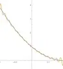
- $I_{c}(t)=A\beta e^{-\beta t}\cos(\omega _{d}t+\phi )-A\omega _{d}e^{-\beta t}\sin(\omega _{d}t+\phi )$
- It turns out that in practice, the attenuation $\beta$ is very small, so $\omega _{d}\approx \omega _{0}.$ This approximation gets better the smaller $\beta$ is.
- This form of the solution, a linear combination of sine and cosine, suggests that we can again rewrite the solution in terms of just one term. Note that the amplitude and phase factor are mathematically different from the previous term, but as we are not given initial conditions, there is no physical difference.
  - $I_{c}(t)=Ae^{-\beta t}\cos(\omega _{d}t+\phi )$

Part 2

Part 2 of 3:

Sinusoidal Voltage Source

1
Consider a sinusoidal voltage source. This voltage source is in the form $V(t)=V_{0}\cos \omega t,$ $V(t)=V_{{0}}\cos \omega t,$ where $V_{0}$ $V_{{0}}$ is the amplitude of the voltage and $\omega$ $\omega$ is the frequency of the signal. The differential equation is now inhomogeneous. By linearity, any solution to the inhomogeneous equation added to the complementary solution gives the general solution.
- ${\ddot {Q}}+2\beta {\dot {Q}}+\omega _{0}^{2}Q={\frac {V_{0}}{L}}\cos \omega t$
2
Use the method of undetermined coefficients to find the particular solution. From the theory of differential equations, we compare the source term to $Q_{c}$ $Q_{{c}}$ and find if the source contains a term that is $t^{n}$ $t^{{n}}$ times a term in $Q_{c}$ $Q_{{c}}$ or not, where $n$ $n$ is 0 or a positive integer. Because there aren't any, the particular solution will take on the following form.
- $Q_{p}=a\cos \omega t+b\sin \omega t$
3
Substitute $Q_{p}$ into the differential equation and equate the two coefficients.
- After some algebra and comparing the coefficients of $\cos \omega t$ $\cos \omega t$ and $\sin \omega t,$ $\sin \omega t,$ we arrive at a system of algebraic equations.
  - $-\omega ^{2}a+2\beta \omega b+\omega _{0}^{2}a={\frac {V_{0}}{L}}$
  - $-\omega ^{2}b-2\beta \omega a+\omega _{0}^{2}b=0$
- These two equations can be written in a more suggestive form.
  - $(\omega _{0}^{2}-\omega ^{2})a+(2\beta \omega )b={\frac {V_{0}}{L}}$
  - $(-2\beta \omega )a+(\omega _{0}^{2}-\omega ^{2})b=0$
4
Solve for the coefficients. We solve for $b$ $b$ in terms of $a,$ $a,$ find $a,$ $a,$ then find $b$ $b$ as a result.
- Use the second equation to solve for $b$ $b$ in terms of $a.$ $a.$
  - $b={\frac {(2\beta \omega )a}{\omega _{0}^{2}-\omega ^{2}}}$
- Substitute back into the first equation to find $a.$ $a.$
  - $(\omega _{0}^{2}-\omega ^{2})a+{\frac {4\beta ^{2}\omega ^{2}}{\omega _{0}^{2}-\omega ^{2}}}a={\frac {V_{0}}{L}}$
  - $a={\frac {{\frac {V_{0}}{L}}(\omega _{0}^{2}-\omega ^{2})}{(\omega _{0}^{2}-\omega ^{2})^{2}+4\beta ^{2}\omega ^{2}}}$
- From here, we immediately find $b.$ $b.$
  - $b={\frac {2\beta \omega V_{0}/L}{(\omega _{0}^{2}-\omega ^{2})^{2}+4\beta ^{2}\omega ^{2}}}$
5
Arrive at the general solution. The coefficients give us the terms that we need in the steady-state solution. The general solution is now simply the sum of the transient and steady-state solutions.
- ${\begin{aligned}Q(t)&=Ae^{-\beta t}\cos(\omega _{d}t+\phi )+{\frac {{\frac {V_{0}}{L}}(\omega _{0}^{2}-\omega ^{2})}{(\omega _{0}^{2}-\omega ^{2})^{2}+4\beta ^{2}\omega ^{2}}}\cos \omega t\\&\quad +{\frac {2\beta \omega V_{0}/L}{(\omega _{0}^{2}-\omega ^{2})^{2}+4\beta ^{2}\omega ^{2}}}\sin \omega t\end{aligned}}$

Part 3

Part 3 of 3:

Resonance

1
Assume the ansatz steady-state solution $Q_{p}=Q(\omega )\cos(\omega t+\delta (\omega ))$ . We have already found the steady-state solution in terms of parameters that we know. Our form of the steady-state solution, a linear combination of sine and cosine, suggests that we can also write it in terms of amplitude and phase factor, just as we did with the transient term. As we will shortly see, this provides a more useful formulation with which to analyze resonance.
2
Substitute into the differential equation. Now, we solve for the amplitude $Q(\omega )$ $Q(\omega )$ and phase $\delta (\omega ),$ $\delta (\omega ),$ both functions of the driving frequency $\omega .$ $\omega .$
- We must make use of the following trigonometric identities in our work.
  - $\cos(\omega t+\delta (\omega ))=\cos \omega t\cos \delta (\omega )-\sin \omega t\sin \delta (\omega )$
  - $\sin(\omega t+\delta (\omega ))=\sin \omega t\cos \delta (\omega )+\cos \omega t\sin \delta (\omega )$
- After substituting and making use of the summation identities, we arrive at the following system of equations.
- $-\omega ^{2}Q(\omega )\cos \omega t\cos \delta (\omega )-2\beta \omega Q(\omega )\sin \delta (\omega )+\omega _{0}^{2}Q(\omega )\cos \delta (\omega )={\frac {V_{0}}{L}}$
- $\omega ^{2}Q(\omega )\sin \delta (\omega )-2\beta \omega Q(\omega )\cos \delta (\omega )-\omega _{0}^{2}Q(\omega )\sin \delta (\omega )=0$
3
Solve for the phase factor $\delta (\omega )$ . We can use the second equation to do this.
- $(\omega ^{2}-\omega _{0}^{2})\sin \delta (\omega )=2\beta \omega \cos \delta (\omega )$
- $\tan \delta (\omega )={\frac {2\beta \omega }{\omega ^{2}-\omega _{0}^{2}}}$
- Our previous results suggest that we write out the denominator as $\omega _{0}^{2}-\omega ^{2}.$ $\omega _{{0}}^{{2}}-\omega ^{{2}}.$ The difference is primarily one of bookkeeping.
  - $\delta (\omega )=\tan ^{-1}{\frac {-2\beta \omega }{\omega _{0}^{2}-\omega ^{2}}}$
4
Solve for the amplitude $Q(\omega )$ . We use the first equation to do this.
- To find $\sin \delta (\omega )$ $\sin \delta (\omega )$ and $\cos \delta (\omega ),$ $\cos \delta (\omega ),$ draw a right triangle with angle $\delta ,$ $\delta ,$ adjacent side length $\omega _{0}^{2}-\omega ^{2},$ $\omega _{{0}}^{{2}}-\omega ^{{2}},$ opposite side length $2\beta \omega ,$ $2\beta \omega ,$ and hypotenuse. Make sure to draw the triangle so that $\sin \delta (\omega )$ $\sin \delta (\omega )$ is negative.
  - $\cos \delta (\omega )={\frac {\omega _{0}^{2}-\omega ^{2}}{\sqrt {4\beta ^{2}\omega ^{2}+(\omega _{0}^{2}-\omega ^{2})^{2}}}}$
  - $\sin \delta (\omega )={\frac {-2\beta \omega }{\sqrt {4\beta ^{2}\omega ^{2}+(\omega _{0}^{2}-\omega ^{2})^{2}}}}$
- We now have all the information needed to find $Q(\omega ).$ $Q(\omega ).$
  - $Q(\omega )={\frac {V_{0}/L}{(\omega _{0}^{2}-\omega ^{2})\cos \delta (\omega )-2\beta \omega \sin \delta (\omega )}}$
- After some simplification, we arrive at the following result.
  - $Q(\omega )={\frac {V_{0}/L}{\sqrt {4\beta ^{2}\omega ^{2}+(\omega _{0}^{2}-\omega ^{2})^{2}}}}$
5
Write the steady-state term in terms of current. Current is once again a derivative away. Note that $\tan ^{-1}x$ $\tan ^{{-1}}x$ is an odd function.
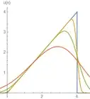
- $I(t,\omega )=-{\frac {\omega V_{0}/L}{\sqrt {4\beta ^{2}\omega ^{2}+(\omega _{0}^{2}-\omega ^{2})^{2}}}}\sin \left(\omega t-\tan ^{-1}{\frac {2\beta \omega }{\omega _{0}^{2}-\omega ^{2}}}\right)$
6
Identify the conditions for resonance.
- Assume that the attenuation is set to 0, or $\beta =0.$ $\beta =0.$ Then the magnitude of the amplitude of the steady-state term is given as the following.
  - $I(\omega )={\frac {\omega V_{0}/L}{\omega _{0}^{2}-\omega ^{2}}}$
- We see that as $\omega \to \omega _{0},$ $\omega \to \omega _{{0}},$ the amplitude increases without bound. This condition is called resonance. An RLC circuit satisfies resonance under the following condition.
  - $\omega =\omega _{0}={\frac {1}{\sqrt {LC}}}$
- The driving force will also have a phase shift of $\pi /2$ $\pi /2$ relative to the steady-state response when resonance is met.
  - $\lim _{\omega \to \omega _{0}}\tan ^{-1}{\frac {-2\beta \omega }{\omega _{0}^{2}-\omega ^{2}}}={\frac {\pi }{2}}$
7
Find the frequency at which maximum amplitude occurs. One only take the derivative, set it to 0, and solve for $\omega .$ $\omega .$ Notice that the $\beta$ $\beta$ term means that the maximum amplitude occurs at a frequency slightly lower than the resonant frequency. But also note that as $\beta$ $\beta$ gets smaller, $\omega _{max}$ $\omega _{{max}}$ gets closer to $\omega _{0}.$ $\omega _{{0}}.$
- ${\dot {Q}}(\omega )=-{\frac {V_{0}}{2L}}(4\beta ^{2}\omega ^{2}+(\omega _{0}^{2}-\omega ^{2})^{2})^{-3/2}(8\beta ^{2}\omega +2(\omega _{0}^{2}-\omega ^{2})(-2\omega ))$
- $8\beta ^{2}\omega -4\omega (\omega _{0}^{2}-\omega ^{2})=0$
- $\omega _{max}={\sqrt {\omega _{0}^{2}-2\beta ^{2}}}$
8
Find the maximum amplitude. Simply substitute our result, and simplify.
- ${\begin{aligned}Q_{max}&={\frac {V_{0}/L}{\sqrt {4\beta ^{2}(\omega _{0}^{2}-2\beta ^{2})+(\omega _{0}^{2}-\omega _{0}^{2}+2\beta ^{2})^{2}}}}\\&={\frac {V_{0}/L}{\sqrt {4\beta ^{2}\omega _{0}^{2}-4\beta ^{4}}}}\\&={\frac {V_{0}/L}{2\beta {\sqrt {\omega _{0}^{2}-\beta ^{2}}}}}\\&={\frac {V_{0}/L}{2\beta \omega _{d}}}\\&={\frac {V_{0}}{R\omega _{d}}}\end{aligned}}$
- We may also write our solution in terms of the amplitude at resonance.
  - $Q_{max}=Q_{res}{\frac {\omega _{0}}{\sqrt {\omega _{0}^{2}-\beta ^{2}}}}$