How to Solve the Heat Equation Using Fourier Transforms

Last Updated: December 2, 2021

The heat equation is a partial differential equation describing the distribution of heat over time. In one spatial dimension, we denote $u(x,t)$ as the temperature which obeys the relation

{\frac {\partial u}{\partial t}}-\alpha {\frac {\partial ^{2}u}{\partial x^{2}}}=0

where $\alpha$ is called the diffusion coefficient. Problems related to partial differential equations are typically supplemented with initial conditions $u(x,0)=u_{0}(x)$ and certain boundary conditions. In this article, we go over how to solve the heat equation using Fourier transforms. It's recommended that you be familiar with their properties before proceeding.

Preliminaries

In this article, we use the following convention for the Fourier transform and its inverse. Note that the Fourier transforms are being applied to real space, not time.
- ${\hat {u}}(\xi ,t)=\int _{-\infty }^{\infty }u(x,t)e^{-i\xi x}\mathrm {d} x$
- $u(x,t)={\frac {1}{2\pi }}\int _{-\infty }^{\infty }{\hat {u}}(\xi ,t)e^{i\xi x}\mathrm {d} \xi$
Diffusion problems frequently encounter the error function, a special function defined as the antiderivative of the Gaussian. The normalization factor is such that the function has a range of $(-1,1).$ $(-1,1).$
- $\operatorname {erf} (x)={\frac {2}{\sqrt {\pi }}}\int _{0}^{x}e^{-t^{2}}\mathrm {d} t$

Steps

1
Transform the equation into Fourier space. In this section, we outline the steps to finding the fundamental solution, a term whose name we will shortly come to understand.
- Taking the Fourier transform of a derivative of order $n$ $n$ is the same as multiplication by $(i\xi )^{n}.$ $(i\xi )^{{n}}.$ Because the Fourier integral is independent of $t,$ $t,$ we can pull the derivative out of the integral and write ${\frac {\partial u}{\partial t}}={\frac {\partial {\hat {u}}}{\partial t}}.$ ${\frac {\partial u}{\partial t}}={\frac {\partial {\hat {u}}}{\partial t}}.$
  - ${\frac {\partial {\hat {u}}}{\partial t}}+\alpha \xi ^{2}{\hat {u}}=0$
2
Solve the resulting ordinary differential equation.
- Solutions are decaying exponentials in $t.$ $t.$ The constant term is the initial conditions in Fourier space, denoted by ${\hat {u}}(\xi ,0)={\hat {u}}_{0}(\xi ).$ ${\hat {u}}(\xi ,0)={\hat {u}}_{{0}}(\xi ).$
  - ${\hat {u}}(\xi ,t)={\hat {u}}_{0}(\xi )e^{-\alpha \xi ^{2}t}$
Advertisement
3
Transform back into real space.
- The property of the Fourier transform we take advantage of here is convolution: multiplication in Fourier space corresponds to convolution in real space.
  - $u(x,t)=u_{0}(x)*U(x,t)$
- The term $U(x,t)={\mathcal {F}}^{-1}\left\{e^{-\alpha \xi ^{2}t}\right\}$ $U(x,t)={\mathcal {F}}^{{-1}}\left\{e^{{-\alpha \xi ^{{2}}t}}\right\}$ is the fundamental solution sought after, also known as the heat kernel. It is the solution to the heat equation given initial conditions of a point source, the Dirac delta function, for the delta function is the identity operator of convolution.
  - $\delta (x)*U(x,t)=U(x,t)$
4
Evaluate the inverse Fourier integral. The inverse Fourier transform here is simply the integral of a Gaussian. We evaluate it by completing the square. If one looks up the Fourier transform of a Gaussian in a table, then one may use the dilation property to evaluate instead.
- ${\begin{aligned}U(x,t)&={\mathcal {F}}^{-1}\left\{e^{-\alpha \xi ^{2}t}\right\}={\frac {1}{2\pi }}\int _{-\infty }^{\infty }e^{-\alpha \xi ^{2}t}e^{ix\xi }\mathrm {d} \xi \\&={\frac {1}{2\pi }}\int _{-\infty }^{\infty }e^{-\alpha t\left(\xi ^{2}-2{\frac {ix\xi }{2\alpha t}}-{\frac {x^{2}}{4\alpha ^{2}t^{2}}}\right)}e^{-x^{2}/4\alpha t}\mathrm {d} \xi \\&={\frac {1}{2\pi }}e^{-x^{2}/4\alpha t}\int _{-\infty }^{\infty }e^{-\alpha t\left(\xi -{\frac {ix}{2\alpha t}}\right)^{2}}\mathrm {d} \xi \\&={\frac {1}{\sqrt {4\pi \alpha t}}}e^{-x^{2}/4\alpha t}\end{aligned}}$
- This is the well-known fundamental solution to the heat equation. From here, we need only substitute initial conditions and evaluate the resulting convolution integral to obtain a solution.
  - $u(x,t)={\frac {1}{\sqrt {4\pi \alpha t}}}\int _{-\infty }^{\infty }u_{0}(y)e^{-(x-y)^{2}/4\alpha t}\mathrm {d} y$
5
Find $u(x,t)$ given initial conditions of the rectangular function.
- The function $u_{0}(x)$ $u_{{0}}(x)$ written below is known by other names, including the gate function, or the unit pulse.
  - $u_{0}(x)={\begin{cases}1&|x|\leq 1/2\\0&|x|>1/2\end{cases}}$
- Now, we simply substitute this function into the convolution integral. Here, the form is particularly simple.
  - ${\begin{aligned}u(x,t)&=\int _{-\infty }^{\infty }u_{0}(y)U(x-y,t)\mathrm {d} y\\&={\frac {1}{\sqrt {4\pi \alpha t}}}\int _{-1/2}^{1/2}e^{-(x-y)^{2}/4\alpha t}\mathrm {d} y\\&={\frac {1}{\sqrt {\pi }}}\int _{z_{-}}^{z_{+}}e^{-z^{2}}\mathrm {d} z,\quad z_{\pm }={\frac {\pm 1/2-x}{\sqrt {4\alpha t}}}\\&={\frac {1}{2}}\left[\operatorname {erf} \left({\frac {1/2-x}{\sqrt {4\alpha t}}}\right)-\operatorname {erf} \left({\frac {-1/2-x}{\sqrt {4\alpha t}}}\right)\right]\end{aligned}}$
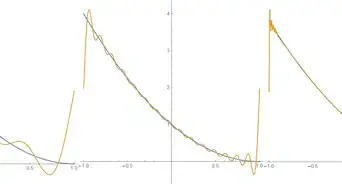
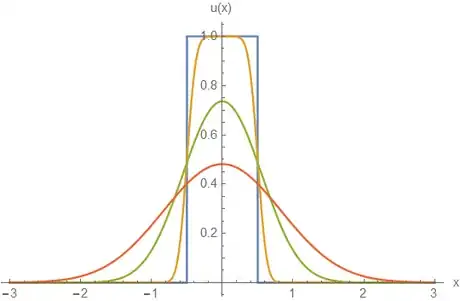
- In the last step, we make use of the fact that $\int e^{-x^{2}}\mathrm {d} x={\frac {\sqrt {\pi }}{2}}\operatorname {erf} (x).$
- A plot of this function over time above shows that the "sharpness" of the function diminishes over time, eventually tending towards an equilibrium solution. This is what the heat equation is supposed to do - it says that the time rate of change of $u(x,t)$ is proportional to the curvature of $u(x,t),$ as denoted by the spatial second derivative, so quantities obeying the heat equation will tend to smooth themselves out over time. The steady-state solution where ${\frac {\partial u}{\partial t}}=0$ will therefore obey Laplace's equation.
- Setting $\alpha =1,$ the initial conditions are plotted in blue, while $u(x,t)$ is being plotted for values $t=0.005,$ $t=0.1,$ and $t=0.3,$ for orange, green, and red plots, respectively.
6
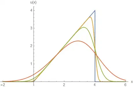
Find $u(x,t)$ given initial conditions of the ramp function over a restricted domain. Specifically, $u_{0}(x)=x(\Theta (x)-\Theta (x-4)),$ $u_{{0}}(x)=x(\Theta (x)-\Theta (x-4)),$ where $\Theta (x)$ $\Theta (x)$ denotes the Heaviside step function. This is the ramp function over the domain $[0,4].$ $[0,4].$ Its solution is slightly more complicated. To find $u(x,t),$ $u(x,t),$ we need to split the integral into two pieces.

${\begin{aligned}u(x,t)&={\frac {1}{\sqrt {4\pi \alpha t}}}\int _{-\infty }^{\infty }y(\Theta (y)-\Theta (y-4))e^{-(x-y)^{2}/4\alpha t}\mathrm {d} y\\&={\frac {1}{\sqrt {4\pi \alpha t}}}\int _{0}^{\infty }ye^{-(x-y)^{2}/4\alpha t}\mathrm {d} y-{\frac {1}{\sqrt {4\pi \alpha t}}}\int _{4}^{\infty }ye^{-(x-y)^{2}/4\alpha t}\mathrm {d} y\end{aligned}}$
- We see that the second integral is different from the first only by the lower boundary. Therefore, we will only detail the process for the first integral only. We make a substitution which splits this integral into two integrals which we may easily evaluate. Note that $u$ below refers to a substitution variable, not to the temperature density.
${\begin{aligned}\int _{0}^{\infty }ye^{-(x-y)^{2}/4\alpha t}\mathrm {d} y&=-{\sqrt {4\alpha t}}\int _{0}^{\infty }\left({\frac {x-y}{\sqrt {4\alpha t}}}\right)e^{\left({\frac {x-y}{\sqrt {4\alpha t}}}\right)^{2}}\mathrm {d} y+x\int _{0}^{\infty }e^{-\left({\frac {x-y}{\sqrt {4\alpha t}}}\right)^{2}}\mathrm {d} y\\&=4\alpha t\int _{x/{\sqrt {4\alpha t}}}^{\infty }ue^{-u^{2}}\mathrm {d} u-x{\sqrt {4\alpha t}}\int _{x/{\sqrt {4\alpha t}}}^{-\infty }e^{-u^{2}}\mathrm {d} u\\&=2\alpha t\int _{x^{2}/4\alpha t}^{\infty }e^{-v}\mathrm {d} v-x{\sqrt {\pi \alpha t}}\operatorname {erf} (u){\Bigg |}_{x/{\sqrt {4\alpha t}}}^{-\infty }\\&=2\alpha te^{-x^{2}/4\alpha t}+x{\sqrt {\pi \alpha t}}\left[1+\operatorname {erf} \left({\frac {x}{\sqrt {4\alpha t}}}\right)\right]\end{aligned}}$
- The second integral is found by a similar process.
$-\int _{4}^{\infty }ye^{-(x-y)^{2}/4\alpha t}\mathrm {d} y=-2\alpha te^{-(x-4)^{2}/4\alpha t}-x{\sqrt {\pi \alpha t}}\left[1+\operatorname {erf} \left({\frac {x-4}{\sqrt {4\alpha t}}}\right)\right]$
- Hence, our final answer is written as follows.
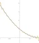
${\begin{aligned}u(x,t)={\sqrt {\frac {\alpha t}{\pi }}}\left(e^{-x^{2}/4\alpha t}-e^{-(x-4)^{2}/4\alpha t}\right)+{\frac {x}{2}}\left[\operatorname {erf} \left({\frac {x}{\sqrt {4\alpha t}}}\right)-\operatorname {erf} \left({\frac {x-4}{\sqrt {4\alpha t}}}\right)\right]\end{aligned}}$
- Setting $\alpha =1,$ the initial conditions are plotted in blue, while $u(x,t)$ is being plotted for values $t=0.01,$ $t=0.1,$ and $t=0.5,$ for orange, green, and red plots, respectively.

Discussion

The heat equation we have been dealing with is homogeneous - that is, there is no source term on the right that generates heat.
- We can show that the total heat is conserved for solutions obeying the homogeneous heat equation. That is, the relation below must be satisfied.
  - $\int _{-\infty }^{\infty }u(x,t)\mathrm {d} x=\int _{-\infty }^{\infty }u_{0}(x)\mathrm {d} x$
- We simply substitute the convolution integral, exchange the order of integration, and then recognize that the integral in $x$ $x$ is simply 1.
  - ${\begin{aligned}\int _{-\infty }^{\infty }u(x,t)\mathrm {d} x&={\frac {1}{\sqrt {4\pi \alpha t}}}\int _{-\infty }^{\infty }\mathrm {d} x\int _{-\infty }^{\infty }u_{0}(y)e^{-(x-y)^{2}/4\alpha t}\mathrm {d} y\\&={\frac {1}{\sqrt {4\pi \alpha t}}}\int _{-\infty }^{\infty }\mathrm {d} x\,e^{-(x-y)^{2}/4\alpha t}\int _{-\infty }^{\infty }\mathrm {d} y\,u_{0}(y)\\&=\int _{-\infty }^{\infty }u_{0}(y)\mathrm {d} y\end{aligned}}$
- Because $y$ is simply a dummy variable, we have shown that the total heat is conserved, as it should be.
A word should be said about the physicality of the solutions that we have obtained.
- The initial conditions describe functions that have compact support. Intuitively, this means that the functions map to non-zero values within some limited domain, and map to zero elsewhere. This is a reasonable description for most materials.
- However, the solutions $u(x,t)$ are defined for $t>0,$ and since the error function is a smooth function over the real line, $u(x,t)$ does not have compact support, implying that the function takes on non-zero values everywhere. We know physically that heat transfer is limited by at least the speed of light, so the model cannot be applied when such conditions become a significant factor. Nevertheless, the solution does decay exponentially, so we may treat the "non-local" regions as an approximation to be neglected.