This article was co-authored by wikiHow staff writer, Jack Lloyd. Jack Lloyd is a Technology Writer and Editor for wikiHow. He has over two years of experience writing and editing technology-related articles. He is technology enthusiast and an English teacher.
The wikiHow Tech Team also followed the article's instructions and verified that they work.
This article has been viewed 479,121 times.
Learn more...
This wikiHow teaches you how to shorten the appearance of data in Microsoft Excel. To do this, your full, unshortened data will need to be entered into Excel first.
Steps
Truncating Text Using the LEFT and RIGHT Formulas
-
1Open Microsoft Excel. If you have an existing document with your data already entered, you can double-click it to open it; otherwise, you'll need to open a new workbook and enter your data now.
-
2Select the cell where you want the truncated text to appear. This method is useful for text that you already have in your spreadsheet.
- Note that this cell must be different than the cell in which your target text appears.
Advertisement -
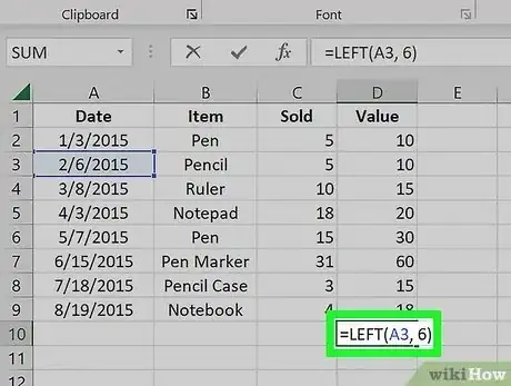
3Type the LEFT or RIGHT formula into your selected cell. The LEFT and RIGHT formula are built on the same premise, though the LEFT formula displays characters from the left side of your cell's text and the RIGHT formula displays characters from the right. The formula is "=DIRECTION(Cell Name, Number of characters to display)" without the quotation marks. For example:[1]
- =LEFT(A3, 6) displays the first six characters in cell A3. If the text in A3 says "Cats are better", the truncated text will read "Cats a" in your selected cell.
- =RIGHT(B2, 5) displays the last 5 characters in cell B2. If the text in B2 says "I love wikiHow", the truncated text will read "kiHow" in your selected cell.
- Keep in mind that spaces count as characters.
-
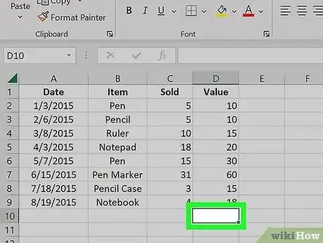
4Press Enter when the formula is complete. Your selected cell will automatically fill with the truncated text.
Truncating Text Using the MID Formula
-
1Select the cell where you want the truncated text to appear. This cell must be different than the cell in which your target text appears.
- If you haven't already added your data to Excel, you'll need to do so first.
-
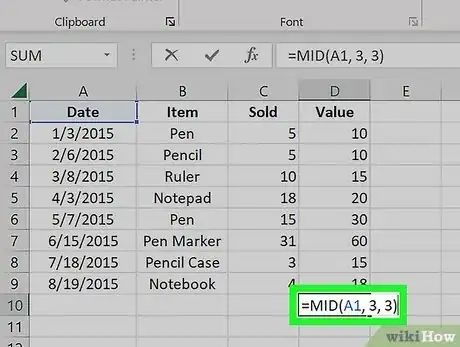
2Type the MID formula into your selected cell. MID chops characters off of the beginning and end of your selected cell's text. To set up the MID formula, you type "=MID(Cell Name, Starting Character Number, Number of characters to display)" without the quotation marks. For example:
- =MID(A1, 3, 3) displays three characters from cell A1, the first of which is the third character from the left in the text. If A1's text says "racecar", the truncated text will read "cec" in your selected cell.
- Similarly, =MID(B3, 4, 8) displays eight characters from cell B3, starting with the fourth character from the left. If B3's text says "bananas aren't people", the truncated text will read "anas are" in your selected cell.
-
3Press Enter when the formula is complete. This will add the truncated text to your selected cell.
Splitting Text Into Multiple Columns
-
1Select the cell you wish to split up. This should be a cell that has more characters than space.
-
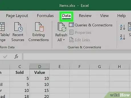
2Click Data. It's in the toolbar at the top of your Excel page.
-
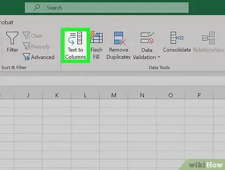
3Select Text to Columns. You'll find this option in the "Data Tools" section of the Data tab.
- This function divides the cell’s contents of one Excel cell into separate columns.
-
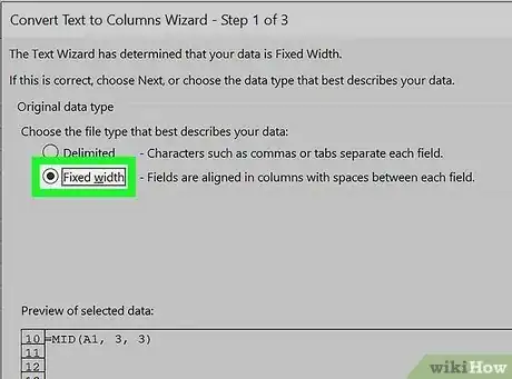
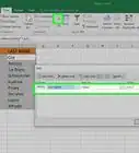
4Select Fixed Width. After clicking on Text to Columns window will pop up, called "Convert Text to Columns Wizard Step 1 of 3." The window will have two selections: "Delimited" and "Fixed Width." Delimited means that characters, such as tabs or commas will divide each field. You will usually select delimited when you’re importing data from another application, such as a database. The fixed width option means that the fields are lined up in columns that have spaces between the individual field.
-
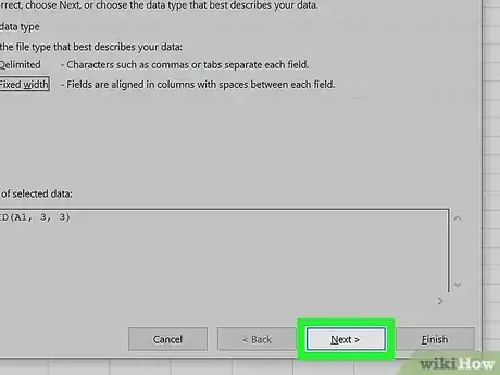
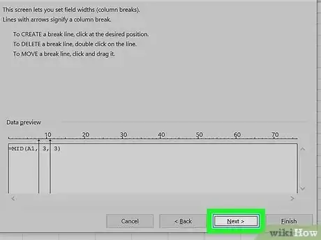
5Click Next. This window shows three options. If you want to create a break line, click on the position where you want the text to break. If you want to delete the break line, double click on the line. To adjust the line, click and drag it around the data.
-
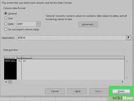
6Click Next. This window has several options, "General", "Text," "Date" and "Do not import column (skip)." Unless you want to force your cell's formatting to do something different than its natural state, you can skip this page.
-
7Click Finish. Your text should now be divided between two or more cells.
Community Q&A
-
QuestionHow do I remove all the text after a period?
 Community AnswerIt depends on whether it is the first period possible, or a later one. I will address it being the first period as the alternatives are a little involved. Use the LEFT() function. The thing you need to work hard for is where is the period? For that, you can use the FIND() function which will locate its position. Since you want precisely that many characters fro the left of the text, nothing more is needed. = LEFT( A1, FIND( ".", A1 ) ). You can use FIND() this way for many things.
 -
QuestionHow can I change all instances of a word to a letter in Excel?
 Community AnswerUse the SUBSTITUTE() function, with the word you wish to change into a letter being the text to go away ("old_text") and the letter you desire in their places being the text to put in place ("new_text").
About This Article
1. Select the cell where you want the truncated text to appear.
2. Type the LEFT or RIGHT formula in the cell.
3. Press Enter.
