This article was co-authored by wikiHow staff writer, Jack Lloyd. Jack Lloyd is a Technology Writer and Editor for wikiHow. He has over two years of experience writing and editing technology-related articles. He is technology enthusiast and an English teacher.
The wikiHow Tech Team also followed the article's instructions and verified that they work.
This article has been viewed 1,952,402 times.
Learn more...
This wikiHow teaches you how to add conditional formatting to a Microsoft Excel spreadsheet on both Windows and Mac computers. Conditional formatting will highlight cells that contain data matching the parameters that you set for the formatting.
Steps
-
1Open your document in Excel. Double-click the Excel spreadsheet that you want to format.
- If you haven't yet created your document, open a new blank spreadsheet in Excel and enter your data before continuing.
-
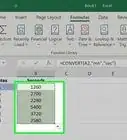
2Select your data. Click and drag your mouse from the top-left cell in your data group to the bottom-right cell in your data group. Your data should now be highlighted.Advertisement
-
3Click the Home tab. It's at the top of the Excel window. This is where you'll find the Conditional Formatting option.
-
4Click Conditional Formatting. You'll find this in the "Styles" section of the Home toolbar. Clicking it prompts a drop-down menu to appear.
-
5Click New Rule…. It's near the bottom of the drop-down menu. Doing so opens the Conditional Formatting window.
-
6Select a rule type. In the "Select a Rule Type" section, click one of the following rules:
- Format all cells based on their values - Applies conditional formatting to every cell in your data. This is the best option for creating a visual gradient when organizing data by average, etc.
- Format only cells that contain - Applies conditional formatting only to cells containing your specified parameters (e.g., numbers higher than 100).
- Format only top or bottom ranked values - Applies conditional formatting to the specified top- or bottom-ranked number (or percentage) of cells.
- Format only values that are above or below average - Applies conditional formatting to cells falling above or below the average as calculated by Excel.
- Format only unique or duplicate values - Applies conditional formatting to either unique or duplicate values.
- Use a formula to determine which cells to format - Applies conditional formatting to cells based on a formula that you have to enter.
-
7Edit your rule. This step will vary based on the rule that you selected:
- Format all cells based on their values - Select a "Minimum" and a "Maximum" value using the drop-down boxes. You can also change the color used for each value in the "Color" drop-down box.
- Format only cells that contain - Select the type of cell that you want to format, then select other rules in the drop-down boxes that appear based on your choice.
- Format only top or bottom ranked values - Select either Top or Bottom, then enter a number of cells to format. You can also enter a percentage number and check the "% of the selected range" box.
- Format only values that are above or below average - Select an above or below average value.
- Format only unique or duplicate values - Select either duplicate or unique in the drop-down box.
- Use a formula to determine which cells to format - Enter your preferred formula in the text box.
-
8Click Format…. It's in the lower-right side of the window. A new window will open.
-
9Click the Fill tab. This tab is in the upper-right side of the new window.
-
10Select a color. Click a color that you want to use for the conditional formatting. This is the color that cells matching your formatting parameters will display.
- Err on the side of light colors (e.g., yellow, light-green, light-blue), as darker colors tend to obscure the text in the cells—especially if you print the document later.
-
11Click OK. It's at the bottom of the window. Doing so closes the "Format" window.
-
12Click OK to apply the formatting. You should see any cells matching your formatting criteria become highlighted with your chosen color.
- If you decide that you want to erase the formatting and start over, click Conditional Formatting, select Clear Rules, and click Clear Rules from Entire Sheet.
-
13Save your spreadsheet. Click File, then click Save to save your changes, or press Ctrl+S (or ⌘ Command+S on a Mac). If you want to save this document as a new document, do the following:
- Windows - Click File, click Save As, double-click This PC, click a save location on the left side of the window, type the document's name into the "File name" text box, and click Save.
- Mac - Click File, click Save As..., enter the document's name in the "Save As" field, select a save location by clicking the "Where" box and clicking a folder, and click Save.


Community Q&A
-
QuestionHow do I get Excel to highlight a particular cell?
 Community AnswerJust click on the particular cell you want to highlight, using the mouse pointer.
 -
QuestionHow do I convert an Excel formula into conditional formatting?Community AnswerIt is not so much converting a formula as using the conditional formatting to display the results of the data (in this case, through a formula). Let's say, for example, you have an entire column (column C) that is the sum of columns A and B. You can apply conditional formatting to column C to search out certain results, like showing cells greater than 10 with a red background.
-
QuestionI have created a sheet to manage my stock levels, I have formatted columns J, K, O, and S to highlight red if the expiry date has been exceeded and green if the expiry date falls within 2 months from today. When there is no date in these columns they show red. I want the columns to stay white. What can I do?
 Community AnswerYou can create a new rule -- "Format only cells that contain", hit "cell value" and choose "blank" instead. Pick whatever formatting you desire. Then ensure this rule is applied first (Applied in Order Shown), and that should solve your problem.
wikiHow Video: How to Apply Conditional Formatting in Excel
Warnings
- Avoid formatting colors or options that make the cells to which they're applied difficult to read.⧼thumbs_response⧽


About This Article
You can use conditional formatting in Excel to automatically add color and style to cells that contain certain values or meet other criteria you define. To get started, open your worksheet in Excel and highlight the cells you want to format. On the Home tab, click the Conditional Formatting button on the toolbar, and then select New Rule from the menu. Now, click the type of rule you'd like to set, and define how it should work. For example, let's say you want all cells containing positive numbers to have blue backgrounds. In this case, you'd choose the Format only cells that contain rule, and then select Cell Value from the first drop-down menu. Select greater than from the next menu, and then type ""0"" into the blank field. Now, let's add the blue background. Click the Format button, and then click the Fill tab. Select a nice light shade of blue from the color palette, and click OK to add it to your rule. If you're happy with your rule, click OK to apply the new formatting conditions to the selected cells.