wikiHow is a “wiki,” similar to Wikipedia, which means that many of our articles are co-written by multiple authors. To create this article, volunteer authors worked to edit and improve it over time.
This article has been viewed 56,328 times.
Learn more...
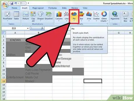
An Excel spreadsheet can be formatted in a variety of ways to perform a number of different tasks. Data can be organized and displayed to suit particular needs, and individual cells can be programmed to make specific calculations based on the data entered. Those calculations can then be inserted into graphical representations of the data, such as charts and graphs. This article provides examples on how to format an Excel spreadsheet to organize, calculate and analyze expenses.
Steps
Format the Expense Tracking Spreadsheet
-
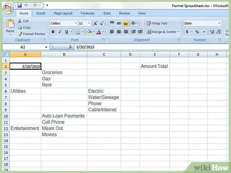
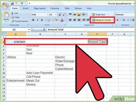
1Format the cells and text. Select cells A2 through E2. Click the Merge and Center button on the Alignment toolbar. Click the Fill Bucket in the Font formatting toolbar and select "White, background 1, Darker 35%."
- Select cells A3 through A5. Press and hold the control key on the computer keyboard and select cells A6 through B9, A10, A11, A12, B12, A13 and B13. Click the Fill Bucket in the Font formatting toolbar and select "White, background 1, Darker 50%."
- Select cells B3 through D3. Press and hold the control key on the computer keyboard and select cells B4 through D4, and B5 through D5. Continue to hold down the control button and select cells B10 through D10, and B11 through D11.
- Click the Fill Bucket in the Font formatting toolbar and select "White, background 1, Darker 50%." Click the Merge and Center button, and the right justify button in the Alignment menu on the toolbar.
- Select cells C6 through D6. Press and hold the control key and select cells C6 through D6, C7 through D7, C8 through D8, and C9 through D9. Click the Fill Bucket and select "White Background 1." With the cells still selected, click the Merge and Center button, and the right justify button in the Alignment menu on the toolbar. Shading and merged cells have been formatted.
-
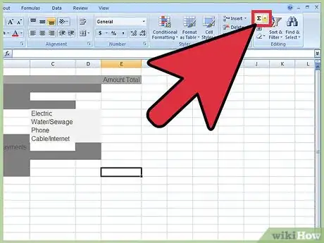
2Program the "Total" cell to add the totals for each category. Click in cell E13 and click the AutoSum button in the editing menu on the far right of the standard toolbar. Select cells E3 through E13 and select the Currency button ($) in the Number formatting menu on the standard toolbar. Numbers entered into the fields for each category will be displayed as a monetary value, and the total will appear at the bottom of the table. The expense tracking sheet has been formatted.
Community Q&A
-
QuestionHow do I format a cell to be the constant in a descending formula?
 Community AnswerPressing f4 locks the reference of a cell. If your formula references the cell after you press f4, it will add $ symbols before the reference. Adding those symbols before both row and column references will lock it in place so that when it starts descending, it will always only reference that cell.
References
- Go with Microsoft, Excel 2007-Comprehensive First Edition, Shelly Gaskin and Karen Jolly. Published in 2008, Pearson Education Inc., Upper Saddle River, NJ.
