How to Row‐Reduce Matrices

Last Updated: November 7, 2020

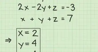
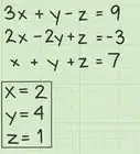
If you have ever taken an algebra course in middle or high school, you’ve probably encountered a problem like this one: solve for $x$ and $y.$

${\begin{aligned}&3x+8y=-33\\&9x+y=-30\end{aligned}}$

These problems are called systems of equations. They often require you to manipulate one of the equations in such a way that you can obtain the values of the other variables. But what if you have 5 equations? Or 50? Or over 200,000, like many problems encountered in real life? That becomes a much more daunting task. Another way to tackle this problem is Gauss-Jordan elimination, or row-reduction.

Part 1

Part 1 of 4:

Setting Up the Matrix

1
Determine if row-reduction is right for the problem. A system of two variables is not very difficult to solve, so row-reducing doesn't have any advantages over substitution or normal elimination. However, this process becomes much slower as the number of equations goes up. Row-reduction allows you to use the same techniques, but in a more systematic way. Below, we consider a system of 4 equations with 4 unknowns.
- ${\begin{aligned}&x_{1}+x_{2}+2x_{3}=1\\&2x_{1}-x_{2}-2x_{4}=-2\\&x_{1}-x_{2}-x_{3}+x_{4}=4\\&2x_{1}-x_{2}+2x_{3}=0\end{aligned}}$
- It is helpful, for purposes of clarity, to align the equations such that by looking from top to bottom, the coefficients of each variable are easily recognized, especially since the variables are only differentiated by subscripts.
2
Understand the matrix equation. The matrix equation $A\mathbf {x} =\mathbf {b}$ $A{\mathbf {x}}={\mathbf {b}}$ is the basic foundation of row-reduction. This equation says that a matrix acting on a vector $\mathbf {x}$ ${\mathbf {x}}$ produces another vector $\mathbf {b} .$ ${\mathbf {b}}.$
- Recognize that we can write the variables and constants as these vectors. Here, $\mathbf {x} =(x_{1},x_{2},x_{3},x_{4}),$ where $\mathbf {x}$ is a column vector. The constants can be written as a column vector $\mathbf {b} .$
- What's left is the coefficients. Here, we put the coefficients into a matrix $A.$ Make sure that every row in the matrix corresponds to an equation, and every column corresponds to a variable.
- ${\begin{pmatrix}1&1&2&0\\2&-1&0&-2\\1&-1&-1&1\\2&-1&2&0\end{pmatrix}}{\begin{pmatrix}x_{1}\\x_{2}\\x_{3}\\x_{4}\end{pmatrix}}={\begin{pmatrix}1\\-2\\4\\0\end{pmatrix}}$
Advertisement
3
Convert your equations into augmented matrix form. As shown, a vertical bar separates the coefficients, written as a matrix $A,$ $A,$ from the constants, written as a vector $\mathbf {b} .$ ${\mathbf {b}}.$ The vertical bar signals the presence of the augmented matrix $(A|\mathbf {b} ).$ $(A|{\mathbf {b}}).$
- $\left({\begin{array}{cccc|c}1&1&2&0&1\\2&-1&0&-2&-2\\1&-1&-1&1&4\\2&-1&2&0&0\end{array}}\right)$

Part 2

Part 2 of 4:

Row-Echelon Form

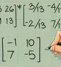
1
Understand elementary row operations. Now that we have the system of equations as a matrix, we need to manipulate it so that we get the desired answer. There are three row operations that we can perform on the matrix without changing the solution. In this step, a row of a matrix will be denoted by $R,$ $R,$ where a subscript will tell us which row it is.
- Row swapping. Simply swap two rows. This is useful in some situations, which we'll get to a bit later. If we want to swap rows 1 and 4, we denote it by $R_{1}\leftrightarrow R_{4}.$
- Scalar multiple. You can replace a row with a scalar multiple of it. For example, if you want to replace row 2 with 5 times itself, you write $R_{2}\to 5R_{2}.$
- Row addition. You can replace a row with the sum of itself and a linear combination of the other rows. If we want to replace row 3 with itself plus twice row 4, we write $R_{3}\to R_{3}+2R_{4}.$ If we want to replace row 2 with itself, plus row 3, plus twice row 4, we write $R_{2}\to R_{2}+R_{3}+2R_{4}.$
- We can do these row operations at the same time, and among the three row operations, the latter two will be the most useful.
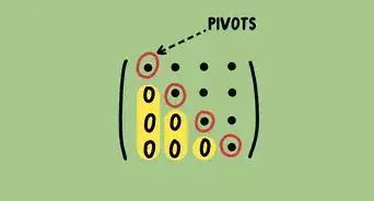
2
Identify the first pivot. A pivot is the leading coefficient of each row. It is unique to each row and column, and identifies a variable with its equation. Let's see how this works.
- In general, the first pivot will always be the top left number, so $x_{1}$ has "its" equation. In our case, the first pivot is the 1 on the top left.
- If the top left number is a 0, swap rows until it is not. In our case, we don't need to.
3
Row-reduce so that everything to the left and bottom of the pivot is 0. When this happens after we have identified all of our pivots, the matrix will be in row-echelon form. The row in which the pivot rests does not change.
- Replace row 2 with itself minus twice row 1. This guarantees that the element in row 2, column 1 will be a 0.
- Replace row 3 with itself minus row 1. This guarantees that the element in row 3, column 1 will be a 0.
- Replace row 4 with itself minus twice row 1. The element in row 4, column 1 will be a 0. Since these row operations pertain to different rows, we can do them simultaneously. There is no need to write out four matrices as part of showing your work.
- These row operations can be summarized below.
- ${\begin{aligned}R_{2}&\to R_{2}-2R_{1}\\R_{3}&\to R_{3}-R_{1}\\R_{4}&\to R_{4}-2R_{1}\end{aligned}}$
- $\left({\begin{array}{cccc|c}1&1&2&0&1\\0&-3&-4&-2&-4\\0&-2&-3&1&3\\0&-3&-2&0&-2\end{array}}\right)$
4
Identify the second pivot and row-reduce accordingly.
- The second pivot can be anything from the second column except that in the first row, because the first pivot already makes it unavailable. Let's choose the element in row 2, column 2. Bear in mind that if a pivot not on the diagonal is chosen, you must row swap so that it is.
- Perform the following row operations such that everything below the pivot is 0.
- ${\begin{aligned}R_{3}&\to 3R_{3}-2R_{2}\\R_{4}&\to R_{4}-R_{2}\end{aligned}}$
- $\left({\begin{array}{cccc|c}1&1&2&0&1\\0&-3&-4&-2&-4\\0&0&-1&7&17\\0&0&2&2&2\end{array}}\right)$
5
Identify the third pivot and row-reduce accordingly.
- The third pivot cannot be from the first or second rows. Let's choose the element in row 3, column 3. Notice a pattern here. We are choosing pivots along the diagonal of the matrix.
- Perform the following row operation. After doing so, the fourth pivot automatically comes out as the lower right element of the matrix.
- $R_{4}\to R_{4}+2R_{3}$
- $\left({\begin{array}{cccc|c}1&1&2&0&1\\0&-3&-4&-2&-4\\0&0&-1&7&17\\0&0&0&16&36\end{array}}\right)$
- This matrix is in row-echelon form now. The pivots have been identified, and everything to the left and below the pivots is 0. Keep in mind that this is a row-echelon form - they are not unique, for different row operations may yield a matrix that looks nothing like the one above.
- You can immediately net $x_{4}={\frac {9}{4}}$ and proceed to substitute to get all other variables. This is called back substitution, and is what computers use after reaching row-echelon form to solve systems of equations. However, we will continue to row-reduce until there stands nothing but the pivots and the constants.

Part 3

Part 3 of 4:

Reduced Row-Echelon Form

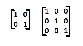
1
Understand what reduced row-echelon form (RREF) is. Unlike ordinary row-echelon, RREF is unique to the matrix, because it requires two additional conditions:
- The pivots are 1.
- The pivots are the only non-zero entry in their respective columns.
- Then, if the system of equations has one unique solution, the resulting augmented matrix will look like $(I|\mathbf {x} ),$ where $I$ is the identity matrix. This is our end goal for this part.
2
Row-reduce to RREF. Unlike obtaining row-echelon form, there is not a systematic process by which we identify pivots and row-reduce accordingly. We just have to do it. It is helpful to simplify before proceeding, however - we can divide row 4 by 4. Doing so makes the arithmetic easier.
- $\left({\begin{array}{cccc|c}1&1&2&0&1\\0&-3&-4&-2&-4\\0&0&-1&7&17\\0&0&0&4&9\end{array}}\right)$
3
Row-reduce such that the third row is all zeroes except for the pivot.
- $R_{3}\to 7R_{4}-4R_{3}$
- $\left({\begin{array}{cccc|c}1&1&2&0&1\\0&-3&-4&-2&-4\\0&0&4&0&-5\\0&0&0&4&9\end{array}}\right)$
4
Row-reduce such that the second row is all zeroes except for the pivot.
- $R_{2}\to R_{3}+R_{2},$ then $R_{2}\to R_{4}+2R_{2}.$ Then simplify the second row.
- $\left({\begin{array}{cccc|c}1&1&2&0&1\\0&-2&0&0&-3\\0&0&4&0&-5\\0&0&0&4&9\end{array}}\right)$
5
Row-reduce such that the first row is all zeroes except for the pivot.
- $R_{1}\to 2R_{1}+R_{2},$ then $R_{1}\to 2R_{1}-R_{3}.$
- $\left({\begin{array}{cccc|c}2&0&0&0&4\\0&-2&0&0&-3\\0&0&4&0&-5\\0&0&0&4&9\end{array}}\right)$
6
Divide so that each pivot is 1.
- $\left({\begin{array}{cccc|c}1&0&0&0&2\\0&1&0&0&3/2\\0&0&1&0&-5/4\\0&0&0&1&9/4\end{array}}\right)$
- This is RREF, and as expected, it immediately gives us the solution to our original equation as $(I|\mathbf {x} ).$ We are now done.
- ${\begin{aligned}x_{1}&=2\\x_{2}&=3/2\\x_{3}&=-5/4\\x_{4}&=9/4\end{aligned}}$

Part 4

Part 4 of 4:

No Unique Solutions

1
Understand the case of inconsistency. The example we went through above had one unique solution. In this part, we go through cases where you encounter a row of 0's in the coefficient matrix.
- After row-reducing as best as you can to row-echelon form, you may encounter a matrix similar to below. The important part is the row with the 0's, but also notice that we lack a pivot in the third row.
- $\left({\begin{array}{ccc|c}1&4&2&1\\0&-4&-1&4\\0&0&0&1\end{array}}\right)$
- That row of 0's says that the linear combination of the variables with coefficients of 0 add up to 1. This is never true, so the system is inconsistent and has no solution. If you reach this point, you are done.
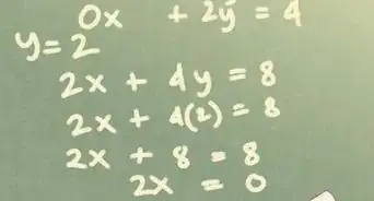
2
Understand the case of dependency. Perhaps in the row of 0's, the constant element in that row is also a 0, like so:
- $\left({\begin{array}{ccc|c}1&4&2&1\\0&-4&-1&4\\0&0&0&0\end{array}}\right)$
- This signals the presence of a dependent solution - a solution set with infinitely many solutions. Some may ask you to stop here, but not every $\mathbf {x}$ is a solution. To see what the actual solution is, row-reduce to RREF.
- $\left({\begin{array}{ccc|c}1&0&1&5\\0&1&1/4&-1\\0&0&0&0\end{array}}\right)$
- The third column lacks a pivot after reducing to RREF, so what does this matrix say exactly? Remember that the pivot "assigns" a row to that variable as its equation, so since the first two rows have pivots, we can identify $x_{1}$ $x_{{1}}$ and $x_{2}.$ $x_{{2}}.$
  - ${\begin{aligned}x_{1}+x_{3}&=5\\x_{2}+{\frac {1}{4}}x_{3}&=-1\end{aligned}}$
- The first equation is the equation for $x_{1},$ $x_{{1}},$ while the second equation is the one for $x_{2}.$ $x_{{2}}.$ Now, solve for both.
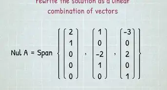
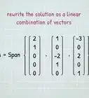
  - ${\begin{aligned}x_{1}&=5-x_{3}\\x_{2}&=-1-{\frac {1}{4}}x_{3}\end{aligned}}$
- This is where "dependency" comes from. Both $x_{1}$ $x_{{1}}$ and $x_{2}$ $x_{{2}}$ rely on $x_{3},$ $x_{{3}},$ but $x_{3}$ $x_{{3}}$ is arbitrary here - it is a free variable. No matter what it is, the resulting pair of $x_{1}$ $x_{{1}}$ and $x_{2}$ $x_{{2}}$ will be a valid solution to the system. To account for this, reparameterize the free variable by setting $x_{3}=t.$ $x_{{3}}=t.$
  - ${\begin{aligned}x_{1}&=5-t\\x_{2}&=-1-{\frac {1}{4}}t\end{aligned}}$
- Of course, plugging in a value for $t$ $t$ and presenting the resulting $\mathbf {x}$ ${\mathbf {x}}$ as a solution does not give the general solution. Rather, the general solution is
  - $\mathbf {x} ={\begin{pmatrix}5-t\\-1-{\frac {1}{4}}t\\t\end{pmatrix}},t\in \mathbb {R} .$
- In general, you may encounter $n$ free variables. In this case, all that is required is that you reparameterize $n$ dependent variables.

Community Q&A

Question

How can I know if the solution is unique or non-unique?

Community Answer

Do the row reduction as usual. If the system has a unique solution, you will get ones along the diagonal and zeros everywhere else. Unique solutions require at least as many equations as unknowns (or columns as rows). If there are infinite solutions, you will find yourself unable to clear one of the columns because there's no pivot for it. This generally happens when you have more unknowns than equations, but can also happen when you thought you had enough equations for a unique solution, but they weren't independent and row reduction simplified one of the equations to 0x + 0y + 0z = 0.