Conway–Maxwell–Poisson distribution
In probability theory and statistics, the Conway–Maxwell–Poisson (CMP or COM–Poisson) distribution is a discrete probability distribution named after Richard W. Conway, William L. Maxwell, and Siméon Denis Poisson that generalizes the Poisson distribution by adding a parameter to model overdispersion and underdispersion. It is a member of the exponential family,[1] has the Poisson distribution and geometric distribution as special cases and the Bernoulli distribution as a limiting case.[2]
|
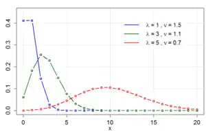
Probability mass function  | |||
|
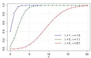
Cumulative distribution function  | |||
| Parameters | |||
|---|---|---|---|
| Support | |||
| PMF | |||
| CDF | |||
| Mean | |||
| Median | No closed form | ||
| Mode | See text | ||
| Variance | |||
| Skewness | Not listed | ||
| Ex. kurtosis | Not listed | ||
| Entropy | Not listed | ||
| MGF | |||
| CF | |||
| PGF | |||
Background
The CMP distribution was originally proposed by Conway and Maxwell in 1962[3] as a solution to handling queueing systems with state-dependent service rates. The CMP distribution was introduced into the statistics literature by Boatwright et al. 2003 [4] and Shmueli et al. (2005).[2] The first detailed investigation into the probabilistic and statistical properties of the distribution was published by Shmueli et al. (2005).[2] Some theoretical probability results of COM-Poisson distribution is studied and reviewed by Li et al. (2019),[5] especially the characterizations of COM-Poisson distribution.
Probability mass function and basic properties
The CMP distribution is defined to be the distribution with probability mass function
where :
The function serves as a normalization constant so the probability mass function sums to one. Note that does not have a closed form.
The domain of admissible parameters is , and , .
The additional parameter which does not appear in the Poisson distribution allows for adjustment of the rate of decay. This rate of decay is a non-linear decrease in ratios of successive probabilities, specifically
When , the CMP distribution becomes the standard Poisson distribution and as , the distribution approaches a Bernoulli distribution with parameter . When the CMP distribution reduces to a geometric distribution with probability of success provided .[2]
For the CMP distribution, moments can be found through the recursive formula [2]
Cumulative distribution function
For general , there does not exist a closed form formula for the cumulative distribution function of . If is an integer, we can, however, obtain the following formula in terms of the generalized hypergeometric function:[6]
The normalizing constant
Many important summary statistics, such as moments and cumulants, of the CMP distribution can be expressed in terms of the normalizing constant .[2][7] Indeed, The probability generating function is , and the mean and variance are given by
The cumulant generating function is
and the cumulants are given by
Whilst the normalizing constant does not in general have a closed form, there are some noteworthy special cases:
- , where is a modified Bessel function of the first kind.[7]
- For integer , the normalizing constant can expressed [6] as a generalized hypergeometric function: .
Because the normalizing constant does not in general have a closed form, the following asymptotic expansion is of interest. Fix . Then, as ,[8]
where the are uniquely determined by the expansion
In particular, , , . Further coefficients are given in.[8]
Moments, cumulants and related results
For general values of , there does not exist closed form formulas for the mean, variance and moments of the CMP distribution. We do, however, have the following neat formula.[7] Let denote the falling factorial. Let , . Then
for .
Since in general closed form formulas are not available for moments and cumulants of the CMP distribution, the following asymptotic formulas are of interest. Let , where . Denote the skewness and excess kurtosis , where . Then, as ,[8]
where
The asymptotic series for holds for all , and .
Moments for the case of integer
When is an integer explicit formulas for moments can be obtained. The case corresponds to the Poisson distribution. Suppose now that . For ,[7]
where is the modified Bessel function of the first kind.
Using the connecting formula for moments and factorial moments gives
In particular, the mean of is given by
Also, since , the variance is given by
Suppose now that is an integer. Then [6]
In particular,
and
Median, mode and mean deviation
Let . Then the mode of is if is not an integer. Otherwise, the modes of are and .[7]
The mean deviation of about its mean is given by [7]
No explicit formula is known for the median of , but the following asymptotic result is available.[7] Let be the median of . Then
as .
Stein characterisation
Let , and suppose that is such that and . Then
Conversely, suppose now that is a real-valued random variable supported on such that for all bounded . Then .[7]
Use as a limiting distribution
Let have the Conway–Maxwell–binomial distribution with parameters , and . Fix and . Then, converges in distribution to the distribution as .[7] This result generalises the classical Poisson approximation of the binomial distribution. More generally, the CMP distribution arises as a limiting distribution of Conway–Maxwell–Poisson binomial distribution.[7] Apart from the fact that COM-binomial approximates to COM-Poisson, Zhang et al. (2018)[9] illustrates that COM-negative binomial distribution with probability mass function
convergents to a limiting distribution which is the COM-Poisson, as .
Related distributions
- , then follows the Poisson distribution with parameter .
- Suppose . Then if , we have that follows the geometric distribution with probability mass function , .
- The sequence of random variable converges in distribution as to the Bernoulli distribution with mean .
Parameter estimation
There are a few methods of estimating the parameters of the CMP distribution from the data. Two methods will be discussed: weighted least squares and maximum likelihood. The weighted least squares approach is simple and efficient but lacks precision. Maximum likelihood, on the other hand, is precise, but is more complex and computationally intensive.
Weighted least squares
The weighted least squares provides a simple, efficient method to derive rough estimates of the parameters of the CMP distribution and determine if the distribution would be an appropriate model. Following the use of this method, an alternative method should be employed to compute more accurate estimates of the parameters if the model is deemed appropriate.
This method uses the relationship of successive probabilities as discussed above. By taking logarithms of both sides of this equation, the following linear relationship arises
where denotes . When estimating the parameters, the probabilities can be replaced by the relative frequencies of and . To determine if the CMP distribution is an appropriate model, these values should be plotted against for all ratios without zero counts. If the data appear to be linear, then the model is likely to be a good fit.
Once the appropriateness of the model is determined, the parameters can be estimated by fitting a regression of on . However, the basic assumption of homoscedasticity is violated, so a weighted least squares regression must be used. The inverse weight matrix will have the variances of each ratio on the diagonal with the one-step covariances on the first off-diagonal, both given below.
Maximum likelihood
The CMP likelihood function is
where and . Maximizing the likelihood yields the following two equations
which do not have an analytic solution.
Instead, the maximum likelihood estimates are approximated numerically by the Newton–Raphson method. In each iteration, the expectations, variances, and covariance of and are approximated by using the estimates for and from the previous iteration in the expression
This is continued until convergence of and .
Generalized linear model
The basic CMP distribution discussed above has also been used as the basis for a generalized linear model (GLM) using a Bayesian formulation. A dual-link GLM based on the CMP distribution has been developed,[10] and this model has been used to evaluate traffic accident data.[11][12] The CMP GLM developed by Guikema and Coffelt (2008) is based on a reformulation of the CMP distribution above, replacing with . The integral part of is then the mode of the distribution. A full Bayesian estimation approach has been used with MCMC sampling implemented in WinBugs with non-informative priors for the regression parameters.[10][11] This approach is computationally expensive, but it yields the full posterior distributions for the regression parameters and allows expert knowledge to be incorporated through the use of informative priors.
A classical GLM formulation for a CMP regression has been developed which generalizes Poisson regression and logistic regression.[13] This takes advantage of the exponential family properties of the CMP distribution to obtain elegant model estimation (via maximum likelihood), inference, diagnostics, and interpretation. This approach requires substantially less computational time than the Bayesian approach, at the cost of not allowing expert knowledge to be incorporated into the model.[13] In addition it yields standard errors for the regression parameters (via the Fisher Information matrix) compared to the full posterior distributions obtainable via the Bayesian formulation. It also provides a statistical test for the level of dispersion compared to a Poisson model. Code for fitting a CMP regression, testing for dispersion, and evaluating fit is available.[14]
The two GLM frameworks developed for the CMP distribution significantly extend the usefulness of this distribution for data analysis problems.
References
- "Conway–Maxwell–Poisson Regression". SAS Support. SAS Institute, Inc. Retrieved 2 March 2015.
- Shmueli G., Minka T., Kadane J.B., Borle S., and Boatwright, P.B. "A useful distribution for fitting discrete data: revival of the Conway–Maxwell–Poisson distribution." Journal of the Royal Statistical Society: Series C (Applied Statistics) 54.1 (2005): 127–142.
- Conway, R. W.; Maxwell, W. L. (1962), "A queuing model with state dependent service rates", Journal of Industrial Engineering, 12: 132–136
- Boatwright, P., Borle, S. and Kadane, J.B. "A model of the joint distribution of purchase quantity and timing." Journal of the American Statistical Association 98 (2003): 564–572.
- Li B., Zhang H., Jiao H. "Some Characterizations and Properties of COM-Poisson Random Variables." Communications in Statistics - Theory and Methods, (2019).
- Nadarajah, S. "Useful moment and CDF formulations for the COM–Poisson distribution." Statistical Papers 50 (2009): 617–622.
- Daly, F. and Gaunt, R.E. " The Conway–Maxwell–Poisson distribution: distributional theory and approximation." ALEA Latin American Journal of Probability and Mathematical Statistics 13 (2016): 635–658.
- Gaunt, R.E., Iyengar, S., Olde Daalhuis, A.B. and Simsek, B. "An asymptotic expansion for the normalizing constant of the Conway–Maxwell–Poisson distribution." To appear in Annals of the Institute of Statistical Mathematics (2017+) DOI 10.1007/s10463-017-0629-6
- Zhang H., Tan K., Li B. "COM-negative binomial distribution: modeling overdispersion and ultrahigh zero-inflated count data." Frontiers of Mathematics in China, 2018, 13(4): 967–998.
- Guikema, S.D. and J.P. Coffelt (2008) "A Flexible Count Data Regression Model for Risk Analysis", Risk Analysis, 28 (1), 213–223. doi:10.1111/j.1539-6924.2008.01014.x
- Lord, D., S.D. Guikema, and S.R. Geedipally (2008) "Application of the Conway–Maxwell–Poisson Generalized Linear Model for Analyzing Motor Vehicle Crashes," Accident Analysis & Prevention, 40 (3), 1123–1134. doi:10.1016/j.aap.2007.12.003
- Lord, D., S.R. Geedipally, and S.D. Guikema (2010) "Extension of the Application of Conway–Maxwell–Poisson Models: Analyzing Traffic Crash Data Exhibiting Under-Dispersion," Risk Analysis, 30 (8), 1268–1276. doi:10.1111/j.1539-6924.2010.01417.x
- Sellers, K. S. and Shmueli, G. (2010), "A Flexible Regression Model for Count Data", Annals of Applied Statistics, 4 (2), 943–961
- Code for COM_Poisson modelling, Georgetown Univ.