Weibull distribution
In probability theory and statistics, the Weibull distribution /ˈwaɪbʊl/ is a continuous probability distribution. It models a broad range of random variables, largely in the nature of a time to failure or time between events. Examples are maximum one-day rainfalls and the time a user spends on a web page.
|
Probability density function 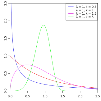 | |||
|
Cumulative distribution function 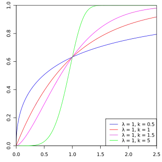 | |||
| Parameters |
scale shape | ||
|---|---|---|---|
| Support | |||
| CDF | |||
| Mean | |||
| Median | |||
| Mode | |||
| Variance | |||
| Skewness | |||
| Ex. kurtosis | (see text) | ||
| Entropy | |||
| MGF | |||
| CF | |||
| Kullback–Leibler divergence | see below | ||
The distribution is named after Swedish mathematician Waloddi Weibull, who described it in detail in 1939,[1] although it was first identified by Maurice René Fréchet and first applied by Rosin & Rammler (1933) to describe a particle size distribution.
Definition
Standard parameterization
The probability density function of a Weibull random variable is[2][3]
where k > 0 is the shape parameter and λ > 0 is the scale parameter of the distribution. Its complementary cumulative distribution function is a stretched exponential function. The Weibull distribution is related to a number of other probability distributions; in particular, it interpolates between the exponential distribution (k = 1) and the Rayleigh distribution (k = 2 and [4]).
If the quantity X is a "time-to-failure", the Weibull distribution gives a distribution for which the failure rate is proportional to a power of time. The shape parameter, k, is that power plus one, and so this parameter can be interpreted directly as follows:[5]
- A value of indicates that the failure rate decreases over time (like in case of the Lindy effect, which however corresponds to Pareto distributions[6] rather than Weibull distributions). This happens if there is significant "infant mortality", or defective items failing early and the failure rate decreasing over time as the defective items are weeded out of the population. In the context of the diffusion of innovations, this means negative word of mouth: the hazard function is a monotonically decreasing function of the proportion of adopters;
- A value of indicates that the failure rate is constant over time. This might suggest random external events are causing mortality, or failure. The Weibull distribution reduces to an exponential distribution;
- A value of indicates that the failure rate increases with time. This happens if there is an "aging" process, or parts that are more likely to fail as time goes on. In the context of the diffusion of innovations, this means positive word of mouth: the hazard function is a monotonically increasing function of the proportion of adopters. The function is first convex, then concave with an inflexion point at .
In the field of materials science, the shape parameter k of a distribution of strengths is known as the Weibull modulus. In the context of diffusion of innovations, the Weibull distribution is a "pure" imitation/rejection model.
First alternative
Applications in medical statistics and econometrics often adopt a different parameterization.[7][8] The shape parameter k is the same as above, while the scale parameter is . In this case, for x ≥ 0, the probability density function is
the cumulative distribution function is
the hazard function is
and the mean is
Second alternative
A second alternative parameterization can also be found.[9][10] The shape parameter k is the same as in the standard case, while the scale parameter λ is replaced with a rate parameter β = 1/λ. Then, for x ≥ 0, the probability density function is
the cumulative distribution function is
and the hazard function is
In all three parameterizations, the hazard is decreasing for k < 1, increasing for k > 1 and constant for k = 1, in which case the Weibull distribution reduces to an exponential distribution.
Properties
Density function
The form of the density function of the Weibull distribution changes drastically with the value of k. For 0 < k < 1, the density function tends to ∞ as x approaches zero from above and is strictly decreasing. For k = 1, the density function tends to 1/λ as x approaches zero from above and is strictly decreasing. For k > 1, the density function tends to zero as x approaches zero from above, increases until its mode and decreases after it. The density function has infinite negative slope at x = 0 if 0 < k < 1, infinite positive slope at x = 0 if 1 < k < 2 and null slope at x = 0 if k > 2. For k = 1 the density has a finite negative slope at x = 0. For k = 2 the density has a finite positive slope at x = 0. As k goes to infinity, the Weibull distribution converges to a Dirac delta distribution centered at x = λ. Moreover, the skewness and coefficient of variation depend only on the shape parameter. A generalization of the Weibull distribution is the hyperbolastic distribution of type III.
Cumulative distribution function
The cumulative distribution function for the Weibull distribution is
for x ≥ 0, and F(x; k; λ) = 0 for x < 0.
If x = λ then F(x; k; λ) = 1 − e−1 ≈ 0.632 for all values of k. Vice versa: at F(x; k; λ) = 0.632 the value of x ≈ λ.
The quantile (inverse cumulative distribution) function for the Weibull distribution is
for 0 ≤ p < 1.
The failure rate h (or hazard function) is given by
The Mean time between failures MTBF is
Moments
The moment generating function of the logarithm of a Weibull distributed random variable is given by[11]
where Γ is the gamma function. Similarly, the characteristic function of log X is given by
In particular, the nth raw moment of X is given by
The mean and variance of a Weibull random variable can be expressed as
and
The skewness is given by
where , which may also be written as
where the mean is denoted by μ and the standard deviation is denoted by σ.
The excess kurtosis is given by
where . The kurtosis excess may also be written as:
Moment generating function
A variety of expressions are available for the moment generating function of X itself. As a power series, since the raw moments are already known, one has
Alternatively, one can attempt to deal directly with the integral
If the parameter k is assumed to be a rational number, expressed as k = p/q where p and q are integers, then this integral can be evaluated analytically.[12] With t replaced by −t, one finds
where G is the Meijer G-function.
The characteristic function has also been obtained by Muraleedharan et al. (2007). The characteristic function and moment generating function of 3-parameter Weibull distribution have also been derived by Muraleedharan & Soares (2014) by a direct approach.
Reparametrization tricks
Fix some . Let be nonnegative, and not all zero, and let be independent samples of , then[13]
- .
Shannon entropy
The information entropy is given by
where is the Euler–Mascheroni constant. The Weibull distribution is the maximum entropy distribution for a non-negative real random variate with a fixed expected value of xk equal to λk and a fixed expected value of ln(xk) equal to ln(λk) − .
Maximum likelihood
The maximum likelihood estimator for the parameter given is
The maximum likelihood estimator for is the solution for k of the following equation[14]
This equation defining only implicitly, one must generally solve for by numerical means.
When are the largest observed samples from a dataset of more than samples, then the maximum likelihood estimator for the parameter given is[14]
Also given that condition, the maximum likelihood estimator for is
Again, this being an implicit function, one must generally solve for by numerical means.
Kullback–Leibler divergence
The Kullback–Leibler divergence between two Weibulll distributions is given by[15]
Weibull plot
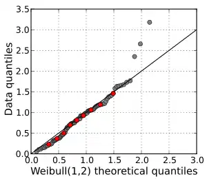
The fit of a Weibull distribution to data can be visually assessed using a Weibull plot.[16] The Weibull plot is a plot of the empirical cumulative distribution function of data on special axes in a type of Q–Q plot. The axes are versus . The reason for this change of variables is the cumulative distribution function can be linearized:
which can be seen to be in the standard form of a straight line. Therefore, if the data came from a Weibull distribution then a straight line is expected on a Weibull plot.
There are various approaches to obtaining the empirical distribution function from data: one method is to obtain the vertical coordinate for each point using where is the rank of the data point and is the number of data points.[17]
Linear regression can also be used to numerically assess goodness of fit and estimate the parameters of the Weibull distribution. The gradient informs one directly about the shape parameter and the scale parameter can also be inferred.
Applications
The Weibull distribution is used
- In survival analysis
- In reliability engineering and failure analysis
- In electrical engineering to represent overvoltage occurring in an electrical system
- In industrial engineering to represent manufacturing and delivery times
- In extreme value theory
- In weather forecasting and the wind power industry to describe wind speed distributions, as the natural distribution often matches the Weibull shape[20]
- In communications systems engineering
- In radar systems to model the dispersion of the received signals level produced by some types of clutters
- To model fading channels in wireless communications, as the Weibull fading model seems to exhibit good fit to experimental fading channel measurements
- In information retrieval to model dwell times on web pages.[21]
- In general insurance to model the size of reinsurance claims, and the cumulative development of asbestosis losses
- In forecasting technological change (also known as the Sharif-Islam model)[22]
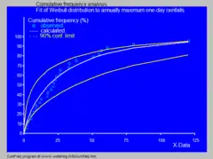
- In hydrology the Weibull distribution is applied to extreme events such as annual maximum one-day rainfalls and river discharges.
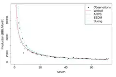
- In decline curve analysis to model oil production rate curve of shale oil wells.[19]
- In describing the size of particles generated by grinding, milling and crushing operations, the 2-Parameter Weibull distribution is used, and in these applications it is sometimes known as the Rosin–Rammler distribution.[23] In this context it predicts fewer fine particles than the log-normal distribution and it is generally most accurate for narrow particle size distributions.[24] The interpretation of the cumulative distribution function is that is the mass fraction of particles with diameter smaller than , where is the mean particle size and is a measure of the spread of particle sizes.
- In describing random point clouds (such as the positions of particles in an ideal gas): the probability to find the nearest-neighbor particle at a distance from a given particle is given by a Weibull distribution with and equal to the density of the particles.[25]
- In calculating the rate of radiation-induced single event effects onboard spacecraft, a four-parameter Weibull distribution is used to fit experimentally measured device cross section probability data to a particle linear energy transfer spectrum.[26] The Weibull fit was originally used because of a belief that particle energy levels align to a statistical distribution, but this belief was later proven false and the Weibull fit continues to be used because of its many adjustable parameters, rather than a demonstrated physical basis.[27]
Related distributions
- A Weibull distribution is a generalized gamma distribution with both shape parameters equal to k.
- The translated Weibull distribution (or 3-parameter Weibull) contains an additional parameter.[11] It has the probability density function
for and for , where is the shape parameter, is the scale parameter and is the location parameter of the distribution. value sets an initial failure-free time before the regular Weibull process begins. When , this reduces to the 2-parameter distribution. - The Weibull distribution can be characterized as the distribution of a random variable such that the random variable
is the standard exponential distribution with intensity 1.[11] - This implies that the Weibull distribution can also be characterized in terms of a uniform distribution: if is uniformly distributed on , then the random variable is Weibull distributed with parameters and . Note that here is equivalent to just above. This leads to an easily implemented numerical scheme for simulating a Weibull distribution.
- The Weibull distribution interpolates between the exponential distribution with intensity when and a Rayleigh distribution of mode when .
- The Weibull distribution (usually sufficient in reliability engineering) is a special case of the three parameter exponentiated Weibull distribution where the additional exponent equals 1. The exponentiated Weibull distribution accommodates unimodal, bathtub shaped[28] and monotone failure rates.
- The Weibull distribution is a special case of the generalized extreme value distribution. It was in this connection that the distribution was first identified by Maurice Fréchet in 1927.[29] The closely related Fréchet distribution, named for this work, has the probability density function
- The distribution of a random variable that is defined as the minimum of several random variables, each having a different Weibull distribution, is a poly-Weibull distribution.
- The Weibull distribution was first applied by Rosin & Rammler (1933) to describe particle size distributions. It is widely used in mineral processing to describe particle size distributions in comminution processes. In this context the cumulative distribution is given by
where- is the particle size
- is the 80th percentile of the particle size distribution
- is a parameter describing the spread of the distribution
- Because of its availability in spreadsheets, it is also used where the underlying behavior is actually better modeled by an Erlang distribution.[30]
- If then (Exponential distribution)
- For the same values of k, the Gamma distribution takes on similar shapes, but the Weibull distribution is more platykurtic.
- From the viewpoint of the Stable count distribution, can be regarded as Lévy's stability parameter. A Weibull distribution can be decomposed to an integral of kernel density where the kernel is either a Laplace distribution or a Rayleigh distribution :
where is the Stable count distribution and is the Stable vol distribution.
See also
References
- Bowers, et. al. (1997) Actuarial Mathematics, 2nd ed. Society of Actuaries.
- Papoulis, Athanasios Papoulis; Pillai, S. Unnikrishna (2002). Probability, Random Variables, and Stochastic Processes (4th ed.). Boston: McGraw-Hill. ISBN 0-07-366011-6.
- Kizilersu, Ayse; Kreer, Markus; Thomas, Anthony W. (2018). "The Weibull distribution". Significance. 15 (2): 10–11. doi:10.1111/j.1740-9713.2018.01123.x.
- "Rayleigh Distribution – MATLAB & Simulink – MathWorks Australia". www.mathworks.com.au.
- Jiang, R.; Murthy, D.N.P. (2011). "A study of Weibull shape parameter: Properties and significance". Reliability Engineering & System Safety. 96 (12): 1619–26. doi:10.1016/j.ress.2011.09.003.
- Eliazar, Iddo (November 2017). "Lindy's Law". Physica A: Statistical Mechanics and Its Applications. 486: 797–805. Bibcode:2017PhyA..486..797E. doi:10.1016/j.physa.2017.05.077. S2CID 125349686.
- Collett, David (2015). Modelling survival data in medical research (3rd ed.). Boca Raton: Chapman and Hall / CRC. ISBN 978-1439856789.
- Cameron, A. C.; Trivedi, P. K. (2005). Microeconometrics : methods and applications. p. 584. ISBN 978-0-521-84805-3.
- Kalbfleisch, J. D.; Prentice, R. L. (2002). The statistical analysis of failure time data (2nd ed.). Hoboken, N.J.: J. Wiley. ISBN 978-0-471-36357-6. OCLC 50124320.
- Therneau, T. (2020). "A Package for Survival Analysis in R." R package version 3.1.
- Johnson, Kotz & Balakrishnan 1994
- See (Cheng, Tellambura & Beaulieu 2004) for the case when k is an integer, and (Sagias & Karagiannidis 2005) for the rational case.
- Balog, Matej; Tripuraneni, Nilesh; Ghahramani, Zoubin; Weller, Adrian (2017-07-17). "Lost Relatives of the Gumbel Trick". International Conference on Machine Learning. PMLR: 371–379.
- Sornette, D. (2004). Critical Phenomena in Natural Science: Chaos, Fractals, Self-organization, and Disorder..
- Bauckhage, Christian (2013). "Computing the Kullback-Leibler Divergence between two Weibull Distributions". arXiv:1310.3713 [cs.IT].
- "1.3.3.30. Weibull Plot". www.itl.nist.gov.
- Wayne Nelson (2004) Applied Life Data Analysis. Wiley-Blackwell ISBN 0-471-64462-5
- "CumFreq, Distribution fitting of probability, free software, cumulative frequency".
- Lee, Se Yoon; Mallick, Bani (2021). "Bayesian Hierarchical Modeling: Application Towards Production Results in the Eagle Ford Shale of South Texas". Sankhya B. 84: 1–43. doi:10.1007/s13571-020-00245-8.
- "Wind Speed Distribution Weibull – REUK.co.uk". www.reuk.co.uk.
- Liu, Chao; White, Ryen W.; Dumais, Susan (2010-07-19). Understanding web browsing behaviors through Weibull analysis of dwell time. ACM. pp. 379–386. doi:10.1145/1835449.1835513. ISBN 9781450301534. S2CID 12186028.
- Sharif, M.Nawaz; Islam, M.Nazrul (1980). "The Weibull distribution as a general model for forecasting technological change". Technological Forecasting and Social Change. 18 (3): 247–56. doi:10.1016/0040-1625(80)90026-8.
- Computational Optimization of Internal Combustion Engine page 49
- Austin, L. G.; Klimpel, R. R.; Luckie, P. T. (1984). Process Engineering of Size Reduction. Hoboken, NJ: Guinn Printing Inc. ISBN 0-89520-421-5.
- Chandrashekar, S. (1943). "Stochastic Problems in Physics and Astronomy". Reviews of Modern Physics. 15 (1): 86.
- ECSS-E-ST-10-12C – Methods for the calculation of radiation received and its effects, and a policy for design margins (Report). European Cooperation for Space Standardization. November 15, 2008.
- L. D. Edmonds; C. E. Barnes; L. Z. Scheick (May 2000). "8.3 Curve Fitting". An Introduction to Space Radiation Effects on Microelectronics (PDF) (Report). NASA Jet Propulsion Laboratory, California Institute of Technology. pp. 75–76.
- "System evolution and reliability of systems". Sysev (Belgium). 2010-01-01.
- Montgomery, Douglas (2012-06-19). Introduction to statistical quality control. [S.l.]: John Wiley. p. 95. ISBN 9781118146811.
- Chatfield, C.; Goodhardt, G.J. (1973). "A Consumer Purchasing Model with Erlang Interpurchase Times". Journal of the American Statistical Association. 68 (344): 828–835. doi:10.1080/01621459.1973.10481432.
Bibliography
- Fréchet, Maurice (1927), "Sur la loi de probabilité de l'écart maximum", Annales de la Société Polonaise de Mathématique, Cracovie, 6: 93–116.
- Johnson, Norman L.; Kotz, Samuel; Balakrishnan, N. (1994), Continuous univariate distributions. Vol. 1, Wiley Series in Probability and Mathematical Statistics: Applied Probability and Statistics (2nd ed.), New York: John Wiley & Sons, ISBN 978-0-471-58495-7, MR 1299979
- Mann, Nancy R.; Schafer, Ray E.; Singpurwalla, Nozer D. (1974), Methods for Statistical Analysis of Reliability and Life Data, Wiley Series in Probability and Mathematical Statistics: Applied Probability and Statistics (1st ed.), New York: John Wiley & Sons, ISBN 978-0-471-56737-0
- Muraleedharan, G.; Rao, A.D.; Kurup, P.G.; Nair, N. Unnikrishnan; Sinha, Mourani (2007), "Modified Weibull Distribution for Maximum and Significant Wave Height Simulation and Prediction", Coastal Engineering, 54 (8): 630–638, doi:10.1016/j.coastaleng.2007.05.001
- Rosin, P.; Rammler, E. (1933), "The Laws Governing the Fineness of Powdered Coal", Journal of the Institute of Fuel, 7: 29–36.
- Sagias, N.C.; Karagiannidis, G.K. (2005). "Gaussian Class Multivariate Weibull Distributions: Theory and Applications in Fading Channels". IEEE Transactions on Information Theory. 51 (10): 3608–19. doi:10.1109/TIT.2005.855598. MR 2237527. S2CID 14654176.
- Weibull, W. (1951), "A statistical distribution function of wide applicability" (PDF), Journal of Applied Mechanics, 18 (3): 293–297, Bibcode:1951JAM....18..293W, doi:10.1115/1.4010337.
- "Weibull Distribution". Engineering statistics handbook. National Institute of Standards and Technology. 2008.
- Nelson Jr, Ralph (2008-02-05). "Dispersing Powders in Liquids, Part 1, Chap 6: Particle Volume Distribution". Retrieved 2008-02-05.