How to Do Curve Fitting in MatLab

Last Updated: December 23, 2021

Curve fitting is an important tool when it comes to developing equations that best describe a set of given data points. Curve fitting is also very useful in predicting the value at a given point through extrapolation. In MATLAB, we can find the coefficients of that equations to the desired degree and graph the curve. If you're not sure how to make a curve fitting in MATLAB, don't worry. This article will walk you through the process step by step.

Part 1

Part 1 of 3:

Getting MATLAB Ready

1
Open MATLAB and click on the New Script button on the left side of the Home tab. Creating the script will help to store your work in a program and will allow reusability.^{[1]
X
Research source}
2
Type commands 'clc' and 'clear all' in the command window. These commands are used to clear the command window and the workspace before executing the script program.

Advertisement
3
Save the script. Click on Save as from the drop-down menu under Save from the editor tab. Name your file and choose the destination file. Then click Save.

Part 2

Part 2 of 3:

Getting Coefficients of the Equation

1
Choose variable and type the data. Choose your independent variable for example ‘x’ and dependent variable for example ‘y’. You can choose any letter for these variables. Write the data points in the square brackets in following format: x = [ ], y = [ ]. Both of these variables are followed by a semicolon (;) if you want to suppress them from appearing in the command window.
2
Import the file if data is in an excel sheet. If you have your data in excel file import the data into MATLAB. You can select the columns from the data that are independent or dependent.
- Click on 'Import Data' from the home tab.
3
Type the file name given file and then click open.
4
Choose the Output type to be 'Column Vector'. This will allow you to choose the independent or dependant vector in the form of a column.
- Select the Columns from the data set.
- At last Click on 'Import Selection' from the tab. Once imported the data columns will show up in the workspace.
5
Choose the independent and dependent variable for the selected data points. The variables chosen should contain the same title as of imported data points. The syntax will be: x = [Column Title]. This same rule applies to the other selected column. Once you have the dependant and independent variable data points we can then use polyfit to find the coefficients.
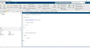
6
Use Polyfit command to get the coefficients of the equation. Polyfit command not only gives coefficients but also lets us choose the highest power of the equation.
- Use the following syntax for the polyfit command, p = polyfit(x,y,n); where x is the independent variable, y is the dependent variable, and n is the degree of the polynomial.

Part 3

Part 3 of 3:

Plotting the Line of Best Fit

1
Use 'polyval' to get the values at the given interval. The syntax of the polyval command is yfit = polyval(p,x), where p is the coefficients of the equation, and x is a vector of independent data points.^{[2]
X
Research source}
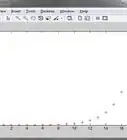
2
Plot the line of best fit. Use the syntax plot (m,yfit) to plot the line of the best fit. You can also add the color of the line by adding 'color initial' in the plot command. For example, plot(x,y,'r'), where 'r' is the color.
- Add the title and axis labels in the plot.
- You can also add the previous plot to the same graph by using function hold on.
- If you need help with any command type help command name in the command window.
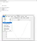
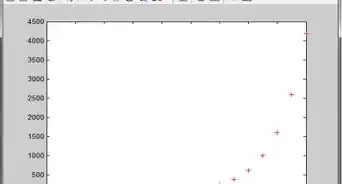
3
Get the results. Click run to see the result.