This article was co-authored by wikiHow staff writer, Nicole Levine, MFA. Nicole Levine is a Technology Writer and Editor for wikiHow. She has more than 20 years of experience creating technical documentation and leading support teams at major web hosting and software companies. Nicole also holds an MFA in Creative Writing from Portland State University and teaches composition, fiction-writing, and zine-making at various institutions.
This article has been viewed 200,725 times.
Learn more...
You can use pivot tables in Excel and Google Sheets to group and organize data in a spreadsheet. Adding rows to a pivot table is as simple as dragging fields into the "Rows" area of your pivot table formatting panel. We'll show you how to add new rows to an existing pivot table in both Microsoft Excel and Google Sheets.
Steps
Microsoft Excel
-
1Review your source data. Click the tab that contains the data you're using in your pivot table, and make sure it contains the data you want to use to create your new row.
- For example, if you want to add a row for a specific purchase, make sure that purchase is listed in the appropriate column in your source data.
-
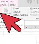
2Click any cell in the PivotTable. This opens the PivotTable Fields panel on the right side of Excel.
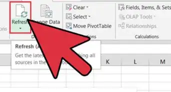
- If you have already moved the appropriate field to the Rows area but don't see a row that's in your source data, just press Alt + F5 or right-click the pivot table and select Refresh.
Advertisement -
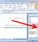
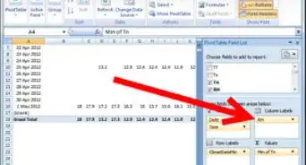
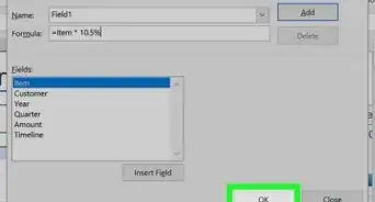
3Drag a field into the "Rows" area on PivotTable Fields. When you drag any of the fields in the upper portion of the PivotTable Fields panel to Rows, a new row will be added to your table.
- Rows are usually non-numeric fields, such as column headers. Numbers will usually go into the Values area.[1]
-
4Reorder the field labels in the "Row Labels" section. If you already have a field in the Rows area, adding another row below that will nest the new row within the existing row.[2] You can drag the rows up or down to change which row is nested within the other.


Google Sheets
-
1Review your source data. Click the tab that contains the data you're using in your pivot table, and make sure it contains the data you want to use to create your new row.
- For example, if you want to add a row for a specific purchase, make sure that purchase is listed in the appropriate column in your source data.
-
2Click anywhere in your pivot table. This opens the pivot table editor on the right side of Google Sheets.
-
3Click Add under "Rows." It's in the left side of the pivot table editor. A list of fields will expand on the menu.
-
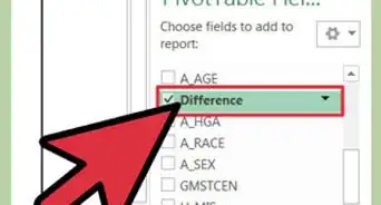
4Click the name of the field you want to add as a row. Rows are usually non-numeric fields, such as category names and/or column headers. Once you select a field, a new row or rows will be added for the items in that field.
- You can also drag any of the labeled fields from the right side of the pivot table panel directly to the Rows area.
-
5Rearrange your rows as needed. If you have multiple rows, adding a new row under an existing row will nest the new row within the existing row. You can drag the row field names up or down to change the order if you want to change the nesting order.


References
About This Article

1. Make sure the info for the row is in your source data.
2. Click the pivot table.
3. Drag a field to the "Rows" area.
4. Reorder rows as needed.