How to Show the Max Value in an Excel Graph

Last Updated: April 12, 2021

This wikiHow will teach you how to show the max value in an Excel graph with a formula. First, you'll need to create a line chart with markers with your data, then you can add a formula to find the maximum of your data set, then you can apply that max to your chart in a new color.

Steps

1
Open your project in Excel. If you're in Excel, you can go to File > Open or you can right-click the file in your file browser.
2
Create a line graph with your data. You'll need to create a line graph for this method to work. To do this, select your data, then go to Insert > Line Graph icon > Line with Markers. It's the line graph with dots.

Advertisement
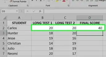
3
Create a new column next to your data set labeled "Max." Since this information will be included in the line graph, keep it close to your original data set so you can easily add it to the data range represented by the graph.
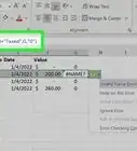
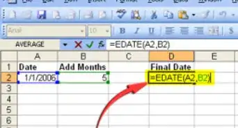
4
Enter the following formula: =IF(B5=MAX($B$5:$B$16),B5,””). In this example, B5 represents the first cell in your range, while B16 represents the last. Replace these cell addresses with the actual cells in your data. This formula will make the highest value in your dataset repeat in this new column, but none of the other values will appear.
- Fill the rest of the column with that formula and you'll see the highest value in your data set repeats in that column.
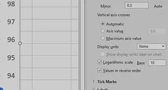
5
Add the "Max" column to your chart. Click your chart to select it, then drag the box highlighting the data it's representing to include the extra column.^{[1]
X
Research source}