This article was co-authored by wikiHow staff writer, Nicole Levine, MFA. Nicole Levine is a Technology Writer and Editor for wikiHow. She has more than 20 years of experience creating technical documentation and leading support teams at major web hosting and software companies. Nicole also holds an MFA in Creative Writing from Portland State University and teaches composition, fiction-writing, and zine-making at various institutions.
This article has been viewed 1,586 times.
Learn more...
Is there a Pivot Table in your Excel workbook that you no longer need? Whether you want to keep the values and calculations created by your Pivot Table or erase it entirely, it's easy to delete Pivot Tables in Excel. This wikiHow article will walk you through two simple ways to delete a Pivot Table from a Microsoft Excel spreadsheet on Windows, Mac, and on the web.
Things You Should Know
- To delete an entire Pivot Table quickly, click anywhere in the table, press Cmd + A (Mac) or Ctrl + A (PC), and then press the Delete key.
- If you want to keep the calculations from your Pivot Table but remove the table formatting, you can copy the data and paste it using Paste Values.
- If you get the error "Cannot change this part of a PivotTable report," click the table, go to PivotTable Analyze > Select > Entire PivotTable, then press Delete.
Steps
Delete the Pivot Table and All Data
-
1Select the entire Pivot Table. If you want to delete your Pivot Table and all of its calculations, start by clicking and dragging your mouse over the entire table to select it. You can also click anywhere inside of the table and press Ctrl + A (PC) or Cmd + A (Mac) to instantly select the whole table.
- If you see an error that says "Cannot change this part of a PivotTable report" or it isn't obvious where your Pivot Table ends or begins, there's another simple way to select the table:
- Click once anywhere in the table.
- Click the PivotTable Analyze tab (or Analyze tab in some versions).
- Click Select on the toolbar.
- Click Entire PivotTable.
- If you see an error that says "Cannot change this part of a PivotTable report" or it isn't obvious where your Pivot Table ends or begins, there's another simple way to select the table:
-
2Press the Del or Delete key. This instantly deletes the entire Pivot Table from your workbook.
- Deleting a Pivot Table won't impact the source data used to create the Pivot Table—you'll only be deleting the contents of the table.[1]
- If your Pivot Table is on its own sheet, you can also simply delete the sheet. To do so, just right-click the sheet's name at the bottom of your workbook and select Delete.


Delete the Table but Keep the Data
-
1Click any cell in the Pivot Table. If you want to keep the data from your Pivot Table but get rid of the Pivot Table itself, you can convert the table to values. Start by clicking any cell in the table.
- Use this method if you created a Pivot Table to perform calculations but now want to work with the data as plain, easy-to-edit text.
-
2Click the PivotTable Analyze tab. You'll see this at the top of Excel.
- Depending on your version of Excel, you might see a "PivotTable Tools" tab with a separate Analyze tab on it. If so, click the Analyze tab.
-
3Click Select on the toolbar. A menu will expand.
-
4Click Entire PivotTable. This selects the entire table, including any data that is filtered out of view.
-
5Right-click the Pivot Table and select Copy. The data is now copied to your clipboard.
-
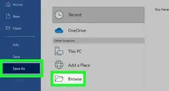
6Click the Home tab. It's at the top-left corner of Excel.
-
7Click the down-arrow below the "Paste" option. You'll see this arrow in the upper-left corner of Excel, below the clipboard icon.
- Don't click the clipboard icon, as you'll get an error. You have to click that arrow just below the icon.
-
8Click the first icon under "Paste Values." It's the small clipboard icon with "123" at the bottom. This replaces the Pivot Table with the selected data.
- Now that you've removed the PivotTable formatting, you can edit the data as needed.
- Considering upgrading your Microsoft 365 account? Check out our coupon site for Staples discounts.


References
About This Article

1. Click any cell in the table.
2. Click the PivotTable Analyze tab.
3. Click Select.
4. Click Entire PivotTable.
5. Right-click the table and select Copy.
6. Click the Home tab.
7. Click the down-arrow under "Paste."
8. Click the first icon under "Paste Values."